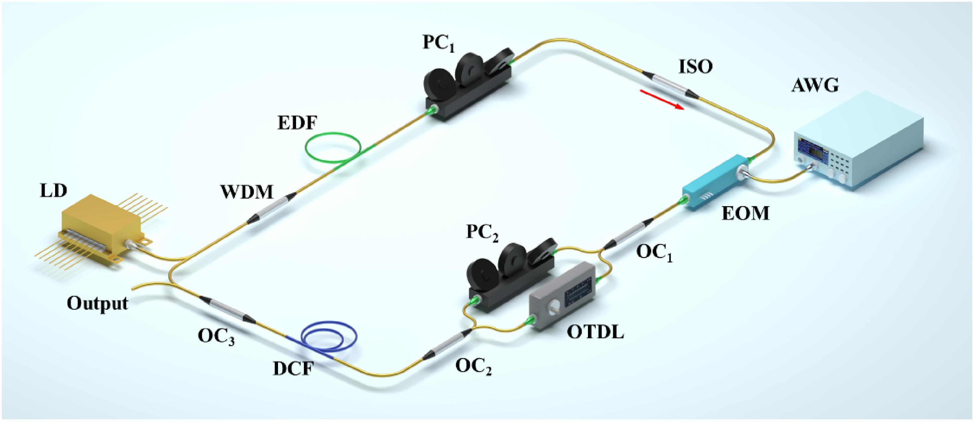
Fig. 1. Laser setup. LD, laser diode; EDF, erbium-doped fiber; WDM, wavelength division multiplexer; ISO, isolator; OC, optical coupler; OTDL, optical time delay line; DCF, dispersion compensating fiber; EOM, electro-optic modulator; AWG, arbitrary waveform generator.

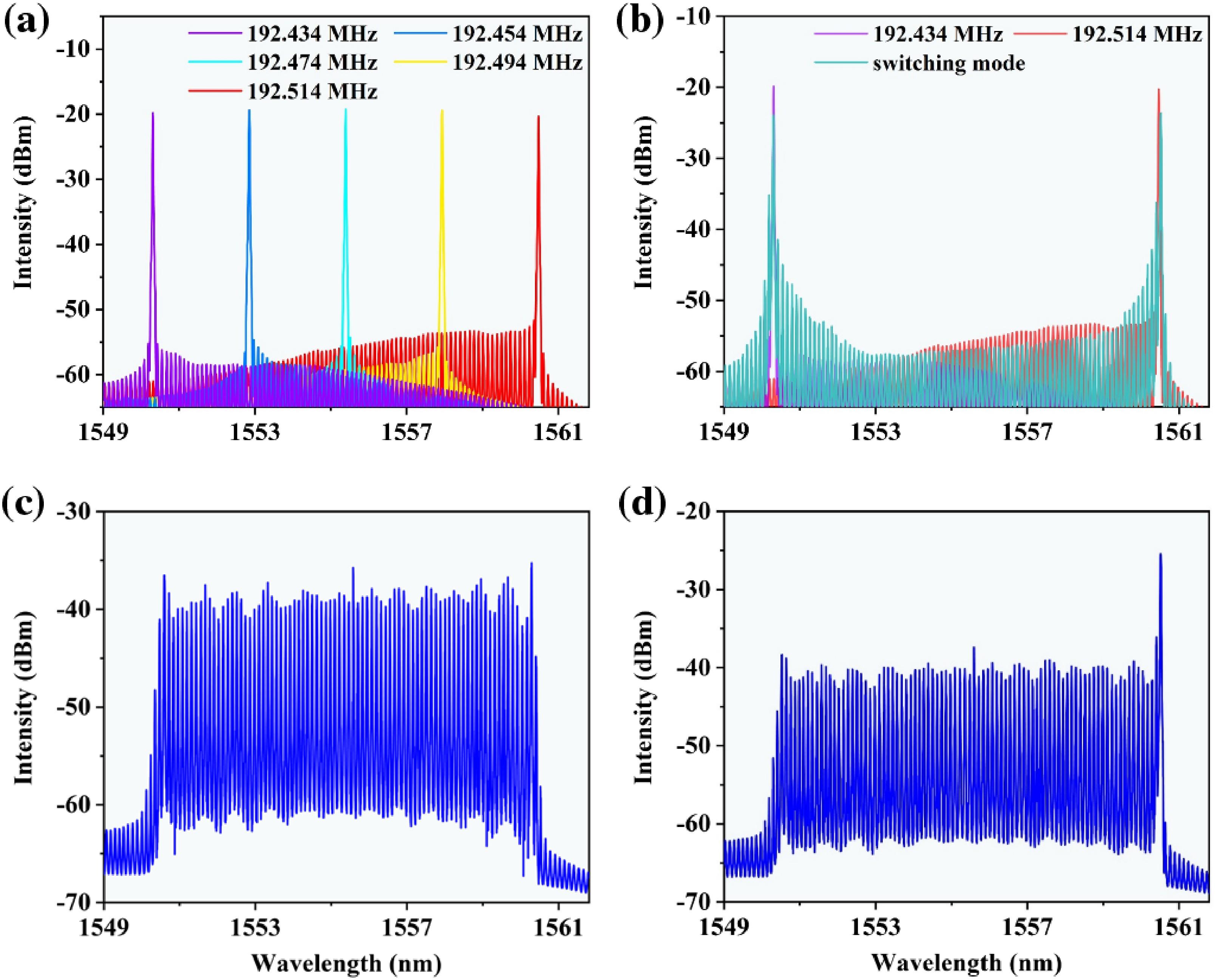
Fig. 2. Spectra of the laser when AWG outputs different sinusoidal signals with various fm. (a) fm is set to 192.434 MHz, 192.454 MHz, 192.474 MHz, 192.494 MHz, and 192.514 MHz, respectively; (b) fm rapidly switches between 192.434 MHz and 192.514 MHz; (c) fm cyclically sweeps between 192.434 MHz and 192.514 MHz; (d) fm is fixed at 192.514 MHz for 2 ms, and then is swept to 192.434 MHz within 2 ms and back to 192.514 MHz within 2 ms. The above process is repeated continuously.

Fig. 3. Experimental results of the fm switching process. (a) Intensity dynamics process measured by a high-speed oscilloscope; (b) the blue curve is the integration of the energy of (a), and the red box corresponds to fm of 192.434 MHz and 192.514 MHz, respectively; (c) close-up of the yellow dashed box in (a); (d) close-up of energy oscillations at RTs=1800–2800 and 4100–5100.

Fig. 4. Experimental results of fm at static and sweep periodic cycles. (a) Real-time pulse evolution is measured by a high-speed oscilloscope; (b) the blue curve is the integration of the energy in (a), and the red wireframes correspond to the states of fm at static, negative sweep (NS), and positive sweep (PS), respectively. (c), (d) Close-up of the yellow dashed boxes in (a), respectively.

Fig. 5. Experimental results of fm at PS and NS cycles. (a) Real-time pulse evolution measured by high-speed oscilloscope; (b) blue curves are the integration of the energy in (a), and red wireframes correspond to the states of fm at PS, NS, and PS, respectively; (c) close-up of the yellow dashed box in (a); (d) variation curves of fm and central wavelength with RTs; the inset is an enlarged view of RTs around 620.

Fig. 6. (a) Principle of MZI-DTSFL; (b) comparison of λc, λs, and λl under different sweeping directions in the experiment.

Fig. 7. (a) Spectra of the laser under different fm when ΔL exceeds 10 cm; (b) characterization of the linewidth of the laser.

Fig. 8. Simulation results. (a) Simulated spectrum evolution in switching mode; (b) the evolution of the pulses corresponding to (a); (c) simulated spectrum evolution in static-sweeping mode; (d) the evolution of the pulses corresponding to (c).

Table 1. Parameters Used in Simulation