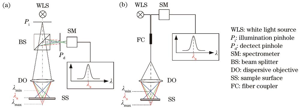
Fig. 1. Schematics of chromatic confocal microscopy. (a) Based on beam splitter; (b) based on fiber coupler

Fig. 2. Schematic diagram of a beam scanning chromatic confocal microscope^[7]

Fig. 3. Schematic diagrams of the line-scanning chromatic confocal sensor^[20]

Fig. 4. Drawing of a chromatic confocal θ-microscope^[24]

Fig. 5. Schematic of the snapshot chromatic confocal matrix sensor^[19]

Fig. 6. Experimental setup and scanning pattern for the microLED-based chromatic confocal microscope^[37]. (a) Experimental setup; (b) schematic pattern of the scanning microLED array

Fig. 7. Schematic diagrams of dispersion focusing and experimental prototype of CCM^[61]. (a) Schematic diagram of the negative dispersion phenomenon of FZP; (b) experimental prototype

Fig. 8. Schematic of a chromatic confocal measurement system^[4]

Fig. 9. Prior self-reference strategy by pre-scanning progress^［44］

Fig. 10. Measurement flowchart with the prior self-reference strategy^［44］

Fig. 11. Fluctuation of peak finding results of different algorithms^［40］. (a) Centroid method; (b) modified centroid method by the interpolation density of 5; (c) modified centroid method by the interpolation density of 9

Fig. 12. Flowchart of mean-shift iterative algorithm

Fig. 13. Schematic of physical slit and virtual slit detection^[81]. (a) Physical slit; (b) virtual slit

Fig. 14. Cross-sectional surface profile of the 8 μm step sample^[37]

Fig. 15. Reconstructed 3D image of an onion epidermis and its volume image^[37]. (a) 3D image; (b) volume image

Fig. 16. Schematic diagrams of line-scanned chromatic confocal microscope^[84]. (a) Optical configuration; (b) prototype system

Fig. 17. Schematic diagrams of the spatially matching image fiber pairs^[84]. (a) Optical configuration of fiber pairs; (b) optimal design of the fiber core diameter and fiber pitch

Fig. 18. Optical system configuration^[33]: (a) DMD-based chromatic confocal microscopic system; (b) DMD projection mode; (c) corresponding CCD sensors

Fig. 19. Light intensity distribution obtained using four different projecting spot sizes^[33]

Fig. 20. Experimental results^[18]. (a) Comparison between the original spectrum signal and the processed signal after one-time deconvolution (the above is the original one while the bottom is the processed one); (b) depth response curves obtained by different number of iterations; (c) relationship between iteration number and FWHM of depth response curve

Fig. 21. Media 1^[92]. (a) CCM image of porcine buccal mucosa; (b) an image of the same tissue from the Lucid Vivascope confocal microscope

Fig. 22. Media 2^[92]. (a) CCM image of porcine buccal mucosa; (b) an image of the same tissue from the Lucid Vivascope confocal microscope

Fig. 23. Schematic of chromatic confocal endoscope^[27]

Fig. 24. Comparison of confocal images in human fingers^[27]. (a) Confocal images of human fingers obtained by CCE; (b)(c) cross-sectional and frontal confocal images of human fingers obtained with a portable confocal microscope

Fig. 25. Cross-section confocal images of human lower lip^[27]. (a) Confocal image of human lower lip internal section obtained by CCE; (b) Frontal confocal image of human lower lip obtained by portable confocal microscope

Fig. 26. System structure and dispersion probe schematic diagram^[94].(a) Schematic of the chromatic confocal system; (b) schematic of the dispersion probe; (c) structure of the annular aperture; (d) the beam of approximately fixed angle of incidence

Fig. 27. Three-dimensional thickness topography of film 3^[94]

Fig. 28. Confocal images acquired with the experimental system^[99]. (a) Standard resolution target; (b) optical section of a microprocessor chip; (c) optical section of the same chip acquired at a different level; (d)-(f) identical to those directly above, however, the optical sectioning strength of the images has been enhanced

Fig. 29. Structural configuration of the on-machine measurement system^[101]

Fig. 30. Schematic presentation of the principle of operation of the optical system^[104]

Fig. 31. The spectral data acquired by the detector in two states^[104].(a) The offline regime; (b) the online regime

Table 1. Performance comparison of different peak extraction algorithms^[42]

Table 2. Thickness measurements of different instruments^[94]

Table 3. Form error parameters of the on-machine and offline measurements^［101］