Researching | Laser Doppler Signal Processing Based on Hybrid Convolution Window

Journals >Laser & Optoelectronics Progress >Volume 60 >Issue 17 >Page 1714008 > Article

Laser & Optoelectronics Progress
Vol. 60, Issue 17, 1714008 (2023)

Laser Doppler Signal Processing Based on Hybrid Convolution Window

Hao Chen^* and Da Zhang

Author Affiliations

College of Automation and Electronic Engineering, Qingdao University of Science and Technology, Qingdao 266061, Shandong , China

show less

DOI: 10.3788/LOP222062 Cite this Article Set citation alerts

Hao Chen, Da Zhang. Laser Doppler Signal Processing Based on Hybrid Convolution Window[J]. Laser & Optoelectronics Progress, 2023, 60(17): 1714008 Copy Citation Text

show less

Sidelobe characteristics of various window functions. (a) Blackman Harris window; (b) four-term Nuttall window; (c) four-term RV window; (d) five-term MSD windows

Fig. 1. Sidelobe characteristics of various window functions. (a) Blackman Harris window; (b) four-term Nuttall window; (c) four-term RV window; (d) five-term MSD windows

Download full size

Sidelobe characteristics of hybrid convolution window functions

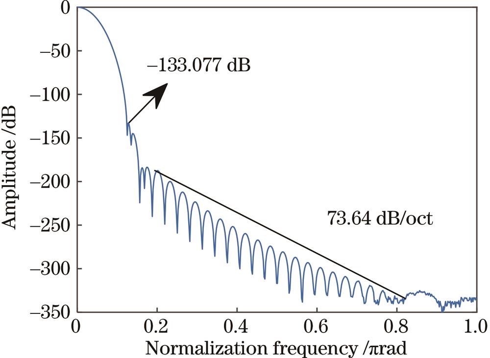
Fig. 2. Sidelobe characteristics of hybrid convolution window functions

Download full size

Fig. 3. Spectral lines. (a) Frequency point is close to the spectral line k₃; (b) frequency point is close to the spectral line k₄; (c) frequency point corresponds to the spectral line; (d) frequency point is in the middle of the two spectral lines

Download full size

Fig. 4. Ideal signals of LDV. (a) Components of the signal; (b) signal time domain waveform

Download full size

Fig. 5. Relative error comparison of frequency detection in low frequency range

Download full size

Fig. 6. Relative error comparison of frequency detection in high frequency range

Download full size

Fig. 7. Signal spectrograms with different signal-to-noise ratios in the low frequency domain. (a) R_SN=+5 dB; (b) R_SN= -5 dB; (c) R_SN=-10 dB; (d) R_SN=-15 dB

Download full size

Fig. 8. Comparison of absolute errors of signal frequency detection with different signal-to-noise ratios in low frequency domain

Download full size

Fig. 9. Signal spectrograms with different signal-to-noise ratios in the high frequency domain. (a) R_SN=+5 dB; (b) R_SN= -5 dB;(c) R_SN= -10 dB; (d) R_SN= -15 dB

Download full size

Fig. 10. Comparison of absolute errors of signal frequency detection with different signal-to-noise ratios in low frequency domain

Download full size

Fig. 11. Comparison of relative errors in low frequency range

Download full size

Fig. 12. Comparison of relative errors in high frequency range

Download full size

Fig. 13. Optical structure of LDV adopted

Download full size

Fig. 14. Experimental setup of LDV

Download full size

Fig. 15. Measured signal sequence

Download full size

Fig. 16. Comparison of relative error of speed

Download full size

No.	Frequency /kHz	Arithmetic mean error of frequency detection /Hz
No.	Frequency /kHz	Method 1	Method 2	Method 3	Method 4
1	60	0.14612	0.03394	0.00311	0.00043
2	120	0.21278	0.05835	0.00570	0.00044
3	180	0.28677	0.06641	0.00946	0.00089
4	240	0.51563	0.11426	0.00709	0.00043
5	300	0.28149	0.06543	0.00928	0.00071
6	360	0.51563	0.11182	0.00803	0.00083
7	420	0.27638	0.06445	0.01013	0.00148
8	480	0.55653	0.10938	0.00791	0.00074
9	540	0.50886	0.06299	0.01247	0.00198
10	600	0.70963	0.10742	0.01038	0.00099
11	660	0.89343	0.06377	0.01201	0.00132
12	720	0.80304	0.06096	0.00916	0.00116
13	780	0.85076	0.06128	0.00707	0.00109
14	840	0.59613	0.05695	0.00713	0.00197
15	900	0.59272	0.06997	0.01402	0.00198

Table 1. Accuracy comparison of frequency detection in low frequency range

No.	Frequency /MHz	Arithmetic mean error of frequency detection /Hz
No.	Frequency /MHz	Method 1	Method 2	Method 3	Method 4
1	60	352.58333	85.10400	5.24102	0.56917
2	120	501.79167	101.60000	11.12227	0.63840
3	180	750.15000	111.82080	11.27520	0.64300
4	240	537.40350	118.33333	12.72240	1.21042
5	300	884.41500	236.29760	28.78092	1.35044
6	360	597.87011	178.52800	18.16214	1.72480
7	420	898.27500	194.54400	29.65572	1.23250
8	480	630.36000	108.39600	15.76973	1.46664
9	540	973.89021	268.07760	28.61121	1.02708
10	600	602.56000	208.08000	16.52556	2.00390
11	660	917.64000	266.31360	31.96869	1.38240
12	720	811.15043	157.22100	19.10038	3.52998
13	780	1289.40000	219.13920	21.50608	2.37312
14	840	805.75000	177.69600	27.56436	2.48270
15	900	902.55010	247.39200	27.11180	3.56040

Table 2. Accuracy comparison of frequency detection in high frequency range

No.	Frequency /kHz	Arithmetical mean of error /Hz
No.	Frequency /kHz	R_SN=+5 dB	R_SN=-5 dB	R_SN=-10 dB	R_SN=-15 dB
1	60	0.00010	0.19175	1.91040	311.33200
2	120	0.00013	0.35768	1.55472	307.64800
3	180	0.00017	0.41007	2.97344	1847.73040
4	240	0.00027	0.74996	2.01240	1923.08880
5	300	0.00017	0.56809	1.59552	1815.69040
6	360	0.00028	0.41415	4.99992	1938.87440
7	420	0.00020	0.73958	11.77808	861.35548
8	480	0.00025	0.90391	9.94064	870.19822
9	540	0.00035	1.19215	19.06470	745.90264
10	600	0.00029	0.93306	10.10534	731.23548
11	660	0.00043	1.18215	30.13222	583.45921
12	720	0.00035	0.93405	26.01698	472.77065
13	780	0.00038	1.12902	21.44346	588.97846
14	840	0.00042	1.11308	26.87693	950.60786
15	900	0.00045	1.05872	30.75494	882.29743

Table 3. Comparison of absolute errors of signal frequency detection with different signal-to-noise ratios in low frequency domain

No.	Frequency /MHz	Arithmetical mean of error /Hz
No.	Frequency /MHz	R_SN =+5 dB	R_SN=-5 dB	R_SN=-10 dB	R_SN=-15 dB
1	60	0.41691	300.48639	1509.27371	454325.23911
2	120	0.49814	338.76866	1228.59782	1768065.17692
3	180	0.92389	526.98932	1369.85067	2385840.38721
4	240	0.97161	405.18828	9136.98548	558740.56227
5	300	0.63717	422.34939	9411.28992	521070.28999
6	360	1.06819	516.84130	9580.61613	446435.45613
7	420	0.79913	786.61318	6553.47962	1287100.12932
8	480	1.04420	531.24111	3526.26674	1313235.31676
9	540	0.97155	574.56118	3147.99428	935988.91351
10	600	0.58315	607.62123	6279.61570	558740.60196
11	660	0.89542	622.92420	9411.28991	521070.30481
12	720	1.10816	796.86612	9580.67975	446435.60156
13	780	0.84019	814.86427	8419.41077	2101635.54417
14	840	1.06821	612.24224	2350.84414	1313235.31558
15	900	0.99453	612.24617	2098.62523	2385350.23874

Table 4. Comparison of absolute errors of signal frequency detection with different signal-to-noise ratios in high frequency domain

No.	Frequency /kHz	Arithmetical mean of error /Hz
No.	Frequency /kHz	FFT	Method 1	Method 2	Method 3	Method4
1	64.5264	4194.14941	4.70772	1.93381	0.32256	0.14568
2	123.1934	4152.20793	7.81245	3.47223	0.56742	0.27769
3	181.8604	4110.68583	8.14860	3.98346	0.84420	0.30182
4	240.5273	4069.57892	11.63889	6.20820	1.20541	0.50791
5	299.1943	4028.88316	15.33006	7.31160	1.59180	0.71136
6	357.8613	3988.59433	13.71006	8.38440	1.42384	0.84032
7	416.5283	3948.70831	17.15013	8.40424	1.77663	0.76533
8	475.1953	3909.22123	18.90783	10.10342	1.96140	1.00400
9	528.9795	3870.12924	20.66472	12.84120	2.15043	0.99814
10	587.6465	3831.42774	24.07887	12.97624	2.49912	0.95342
11	646.3135	3793.11352	22.45887	13.73043	2.33120	1.42140
12	704.9805	3755.18236	25.74423	13.40101	2.67124	1.36353
13	763.6475	3717.63057	29.05551	14.20563	2.84346	1.29140
14	822.3145	3680.45421	32.28012	17.21520	3.17943	1.43463
15	880.9814	3643.64973	33.88392	19.57682	3.51544	1.75682

Table 5. Precision comparisons in low frequency range

No.	Frequency /MHz	Arithmetical mean of error /Hz
No.	Frequency /MHz	FFT	Method 1	Method2	Method3	Method4
1	54.7852	3808593.75686	3997.02938	2036.72159	343.86209	176.33953
2	113.4277	3759765.63471	6352.98234	3237.21821	546.54333	280.27863
3	172.0703	3710937.53730	11860.12172	5385.60410	1020.31929	523.24066
4	230.7129	3662109.38275	17203.43953	6876.16441	1480.00178	641.10807
5	289.3555	3613281.25344	14531.78766	7404.80062	1250.16114	717.94732
6	347.9980	3564453.13781	19756.84712	10067.27940	1699.66994	871.62561
7	416.4063	3515625.69218	24762.72983	12618.06748	2130.32308	1092.47338
8	475.0488	3466796.88477	22310.24485	11368.38211	2949.41357	984.27551
9	528.8086	3417968.75109	27215.20969	13867.75023	2750.42503	1200.67102
10	587.4512	3369140.63511	29592.98431	15079.36627	2279.33724	1305.57284
11	646.0938	3320312.51726	34283.78167	17469.60345	2341.30848	1512.51978
12	704.7363	3271484.38414	31970.75250	16290.97903	2545.86703	1410.47438
13	763.3789	3222656.25844	36596.80313	18648.22394	3148.40145	1614.56484
14	822.0215	3173828.13282	38856.96480	19799.90684	3342.84141	1714.27765
15	880.6641	3125000.11710	41117.10844	20951.58540	3537.28065	1813.99008

Table 6. Precision comparisons in high frequency range

Item	Method 1	Method 2	Method 3	Method 4
Low frequency	0.0044	0.00229	0.00043	0.00020
High frequency	0.0055	0.00273	0.00048	0.00024

Table 7. Relative error averages in the low and high frequency ranges

Wavelength range /nm

Output

bandwidth /MHz

Active area

diameter /mm

Input optical power range /

μ W

400‒1000

400

0.5

8‒80

Table 8. Main parameters of APD 430A/M

No.	Reference speed /（m·s^-1）	Arithmetical mean of error /（m·s^-1）
No.	Reference speed /（m·s^-1）	Method 1	Method 2	Method 3	Method 4
1	0.5415	1.58518×10^-4	8.67780×10^-5	1.88374×10^-5	1.15203×10^-5
2	0.5898	1.79469×10^-4	9.70299×10^-5	1.93083×10^-5	1.18081×10^-5
3	0.6377	2.15047×10^-4	9.78912×10^-5	1.91513×10^-5	1.17123×10^-5
4	0.7056	2.60572×10^-4	9.86931×10^-5	1.93083×10^-5	1.18080×10^-5
5	0.7683	3.14231×10^-4	1.03356×10^-4	2.15460×10^-5	1.19047×10^-5
6	0.8675	3.67119×10^-4	1.12973×10^-4	2.58036×10^-5	1.26724×10^-5
7	0.9369	3.10047×10^-4	1.25720×10^-4	2.78561×10^-5	1.36800×10^-5
8	0.9897	3.36604×10^-4	1.31654×10^-4	2.89313×10^-5	1.77600×10^-5
9	1.0425	2.69283×10^-4	1.17746×10^-4	3.56754×10^-5	1.96536×10^-5
10	1.0832	2.67506×10^-4	1.04587×10^-4	3.69357×10^-5	2.15417×10^-5
11	1.1238	2.56270×10^-4	1.07916×10^-4	4.29600×10^-5	2.21475×10^-5
12	1.1605	2.71244×10^-4	1.36797×10^-4	4.76400×10^-5	2.38255×10^-5
13	1.1972	2.48648×10^-4	1.43981×10^-4	4.76400×10^-5	2.38213×10^-5
14	1.2492	2.39082×10^-4	1.57070×10^-4	4.77600×10^-5	2.38846×10^-5
15	1.2971	2.51415×10^-4	1.70160×10^-4	4.81200×10^-5	2.40676×10^-5

Table 9. Processing results of measured signals

Get PDF(in Chinese)

Figures&Tables (25)

References (20)

Copy Citation Text

Hao Chen, Da Zhang. Laser Doppler Signal Processing Based on Hybrid Convolution Window[J]. Laser & Optoelectronics Progress, 2023, 60(17): 1714008

Download Citation

Set citation alerts for the article

Set citation alerts for the article

Save the article for my favorites

Paper Information

Recommended Topics

laser devices and laser physics

Lasers and Laser Optics

laser manufacturing

Instrumentation, Measurement and Metrology

Set citation alerts for the article

Please enter your email address