Hyperspectral On-Board Classification Algorithm Based on Multiscale Feature Extraction

Shuai Yuan; Yanan Sun; Weifeng He; Shikui Tu

doi:10.3788/LOP213289

Journals >Laser & Optoelectronics Progress >Volume 60 >Issue 10 >Page 1010004 > Article

Laser & Optoelectronics Progress
Vol. 60, Issue 10, 1010004 (2023)

Hyperspectral On-Board Classification Algorithm Based on Multiscale Feature Extraction

Shuai Yuan, Yanan Sun^*, Weifeng He, and Shikui Tu

Author Affiliations

School of Electronic Information and Electrical Engineering, Shanghai Jiao Tong University, Shanghai 200240, China

show less

DOI: 10.3788/LOP213289 Cite this Article Set citation alerts

Shuai Yuan, Yanan Sun, Weifeng He, Shikui Tu. Hyperspectral On-Board Classification Algorithm Based on Multiscale Feature Extraction[J]. Laser & Optoelectronics Progress, 2023, 60(10): 1010004 Copy Citation Text

show less

Fig. 1. Spatial feature extraction method based on multiscale local maximum

Download full size

Classification maps of each algorithm on Indian Pines dataset. (a) Ground truth; (b) SVM; (c) RF; (d) CNN1D; (e) CNN2D; (f) HybridSN; (g) A2S2K-ResNet; (h) LBP-RF; (i) EMP-RF; (j) MF-RF

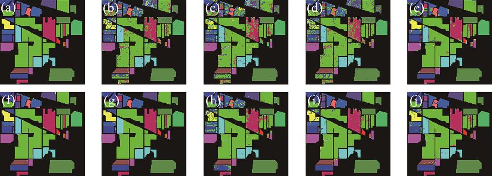
Fig. 2. Classification maps of each algorithm on Indian Pines dataset. (a) Ground truth; (b) SVM; (c) RF; (d) CNN1D; (e) CNN2D; (f) HybridSN; (g) A²S²K-ResNet; (h) LBP-RF; (i) EMP-RF; (j) MF-RF

Download full size

Fig. 3. Classification maps of each algorithm on Pavia University dataset. (a) Ground truth; (b) SVM; (c) RF; (d) CNN1D; (e) CNN2D; (f) HybridSN; (g) A²S²K-ResNet; (h) LBP-RF; (i) EMP-RF; (j) MF-RF

Download full size

Fig. 4. Number of operations in the classification process of each algorithm. (a) Spectral algorithms; (b) one-stage spatial-spectral algorithms; (c) two-stage spatial-spectral algorithms

Download full size

Fig. 5. Energy consumption of each algorithm in the classification process. (a) Spectral algorithms; (b) one-stage spatial-spectral algorithms; (c) two-stage spatial-spectral algorithms

Download full size

Algorithm		Number of operations
Algorithm		Exp	Mul	Add	Cmp
Spectral algorithm（k：number of features，l：number of classes）	SVM	M	kM+2M	kM+l
	SVM	M：number of support vectors
	RF			N	DN
	RF	$D$ ：average depth of trees， $N$ ：number of trees
	CNN1D		$(k - q + 1) q l$	$(k - q + 1) q l$
	CNN1D	$q$ ：number of values in each filter
One-stage spatial-spectral algorithm （K：kernel size， C_in：number of input channels， C_out：number of output channels）	Each convolution layer		$K^{2} \times C_{i n} \times C_{o u t}$	$K^{2} \times C_{i n} \times C_{o u t}$
Two-stage spatial-spectral algorithm（ $k^{'}$ ：number of features）	LBP-RF			$N$	$k^{'} p + D N$
	LBP-RF	$p$ ：number of points in LBP， $D / N$ ：same as RF
	EMP-RF		$M u l (P C A)$	$A d d (P C A) + N$	$\sum_{1}^{m} {S_{i}}^{2} + D N$
	EMP-RF	$M u l (P C A) 、 A d d (P C A)$ ：number of Mul/Add in PCA， $S_{i}$ ：size of each structuring element， $m$ ：number of structuring elements， $D / N$ ：same as RF
	MF-RF			$N$	${(2 r_{m a x} + 1)}^{2} + D N$
	MF-RF	$r_{m a x}$ ：radius of the largest filter， $D / N$ ：same as RF

Table 1. Statistics of operation type and number of operations of different algorithms

Class	Spectral algorithm			One-stage spatial-spectral algorithm			Two-stage spatial-spectral algorithm
Class	SVM	RF	CNN1D	CNN2D	HybridSN	A²S²K-ResNet	LBP-RF	EMP-RF	MF-RF
Alfalfa	81.82	100.00	87.50	100.00	80.49	100.00	95.24	97.83	91.84
Corn-notil	78.91	73.58	73.38	90.24	95.10	97.78	82.34	94.76	95.49
Corn-mintill	80.69	75.93	75.30	90.85	99.46	98.69	88.00	95.17	94.72
Corn	63.14	59.60	79.31	87.98	93.90	96.27	74.05	83.87	93.81
Grass-pasture	92.83	88.70	91.39	93.95	98.16	99.31	97.17	94.00	96.21
Grass-trees	85.24	82.98	94.59	93.98	99.24	99.44	88.18	97.90	95.45
Grass-pasture-mowed	83.87	100.00	95.00	100.00	100.00	92.22	90.00	100.00	89.66
Hay-windrowed	92.59	86.34	93.25	98.73	99.53	99.32	94.43	100.00	97.95
Oats	100.00	100.00	100.00	90.91	61.11	84.65	100.00	100.00	100.00
Soybean-notill	80.05	72.25	82.65	91.12	98.17	97.56	92.16	92.94	95.96
Soybean-mintill	77.97	73.37	69.97	94.80	99.05	99.13	86.45	94.68	96.16
Soybean-clean	77.26	66.60	85.78	92.58	90.26	98.10	87.74	89.64	92.95
Wheat	90.13	90.91	94.34	95.71	95.14	99.20	100.00	100.00	98.51
Woods	93.25	93.06	93.31	96.48	99.47	99.29	99.37	99.21	99.61
Buildings-Grass-Trees-Drives	73.82	58.43	71.70	96.21	95.97	98.00	97.49	94.33	98.21
Stone-Steel-Towers	98.77	98.75	100.00	78.38	90.48	96.30	92.86	97.89	98.78
OA	82.34	77.62	80.11	93.43	97.44	98.57	89.66	95.15	96.26
AA	84.39	82.53	86.72	93.24	93.47	97.20	91.59	95.76	95.96
Kappa	79.75	74.26	77.01	92.50	97.08	98.37	88.14	94.46	95.73

Table 2. Classification results on Indian Pines dataset

Class	Spectral algorithm			One-stage spatial-spectral algorithm			Two-stage spatial-spectral algorithm
Class	SVM	RF	CNN1D	CNN2D	HybridSN	A²S²K-ResNet	LBP-RF	EMP-RF	MF-RF
Asphalt	93.60	92.03	95.15	98.75	100.00	99.76	97.12	99.40	98.68
Meadows	96.17	90.22	98.17	99.33	100.00	99.95	98.65	99.82	99.30
Gravel	88.38	86.50	89.82	97.90	98.68	99.42	96.69	99.86	98.76
Trees	96.25	96.21	95.10	96.19	99.45	99.88	97.10	99.90	99.14
Painted metal sheets	99.04	98.23	99.63	99.56	100.00	99.97	99.48	100.00	99.85
Bare Soil	94.65	92.93	91.94	99.26	100.00	99.96	98.26	99.94	99.80
Bitumen	92.73	86.11	92.05	92.81	100.00	100.00	99.13	99.70	99.62
Self-Blocking Bricks	86.00	82.08	85.33	97.48	99.70	99.00	93.86	99.08	99.17
Shadows	100.00	100.00	99.37	99.55	94.60	100.00	99.79	99.68	99.79
OA	94.41	90.56	95.07	98.58	99.72	99.81	97.81	99.71	99.25
AA	94.09	91.59	94.06	97.87	99.11	99.77	97.79	99.71	99.35
Kappa	92.56	87.26	93.48	98.12	99.63	99.75	97.10	99.62	99.01

Table 3. Classification results on Pavia University dataset

Dataset

Spectral algorithm

One-stage spatial-spectral algorithm

Two-stage spatial-spectral algorithm

SVM

CNN1D

CNN2D

HybridSN

A²S²K-

ResNet

LBP-RF

EMP-RF

MF-RF

Indian Pines

3.41

0.54

1.20

6.11

72.30

45.68

4.38

1.48

1.07

Pavia University

39.23

4.15

7.43

59.56

277.31

117.42

79.70

12.69

16.69

Table 4. Classification times of different algorithms on two datasets

Class	RF	L1+RF	ST+RF	ST+CORAL+RF	MF-RF（17）	ST+CORAL+MF-RF（52）
Dense Urban Fabric	5.78	29.17	4.39	3.70	8.21	15.49
Mineral Extraction Sites	0.00	17.07	16.24	34.09	2.50	33.33
Non-Irrigated Arable Land	25.00	83.14	45.71	92.18	66.67	76.61
Fruit Trees	0.00	0.00	1.52	3.05	0.00	1.96
Olive Groves	2.22	44.44	0.00	81.40	0.00	62.63
Coniferous Forest	100.00	87.50	64.60	39.49	85.71	28.15
Dense Sclerophyllous Vegetation	67.54	67.88	68.45	71.68	66.59	69.38
Sparce Sclerophyllous Vegetation	44.33	37.46	51.43	49.70	45.65	51.60
Sparcely Vegetated Areas	9.38	11.66	4.99	17.28	9.29	17.92
Rocks and Sand	9.45	28.00	56.91	57.32	8.93	58.40
Water	62.28	95.15	100.00	100.00	67.64	100.00
Coastal Water	3.01	100.00	100.00	99.34	2.15	96.16
OA	46.66	51.99	55.45	58.59	48.57	60.03
AA	27.42	50.12	42.85	54.10	30.28	50.97
Kappa	33.13	41.27	45.95	49.92	35.52	50.67

Table 5. Classification results on HyRANK dataset

Dataset	PSNR /dB	RF	CNN1D	MF-RF（minimum）	MF-RF（maximum）
Indian Pines		77.62	80.11	93.76	96.26
	36.38	77.10	80.07	93.27	95.07
	26.38	74.14	76.19	93.04	94.67
Pavia University		90.56	95.07	99.06	99.25
	35.07	89.94	93.61	98.80	99.28
	25.07	85.79	87.77	97.94	99.31

Table 6. Classification results of RF, CNN1D, and MF-RFs based on different feature values

Dataset		MF-SVM	MF-FC	MF-RF
Indian Pines	OA	94.89	79.61	96.26
	AA	95.60	76.72	95.96
	Kappa	94.17	76.62	95.73
Pavia University	OA	99.47	90.46	99.25
	AA	99.49	89.13	99.35
	Kappa	99.29	87.33	99.01

Table 7. Comparison of MF and different classifiers combinations

Dataset		CNN1D-RF	CNN2D-RF	MF-RF
Indian Pines	OA	80.88	92.53	96.26
	AA	87.78	93.65	95.96
	Kappa	77.93	91.44	95.73
Pavia University	OA	95.37	97.93	99.25
	AA	95.19	97.79	99.35
	Kappa	93.83	97.25	99.01

Table 8. Comparison of different CNN feature extraction methods and RF combinations

Operation type	Data precision /bit	Energy cost /pJ
Integer comparison	8	0.008
Floating-point addition	32	0.9
Floating-point multiplication	32	3.7
Floating-point exponentiation	32	38.975

Table 9. Energy consumption of different operation types

Classification algorithm	Indian Pines	Pavia University
SVM	2.8×10⁷	2.4×10⁷
RF	1.0×10²	1.1×10²
CNN1D	7.2×10⁵	3.1×10⁵
CNN2D	1.8×10⁸	1.3×10⁸
HybridSN	1.1×10⁹	1.1×10⁹
A²S²K-ResNet	7.7×10¹⁰	3.8×10¹⁰
LBP-RF	1.1×10²	1.3×10²
EMP-RF	5.4×10⁷	1.8×10⁶
MF-RF	2.7×10²	1.0×10³

Table 10. Energy consumption of each algorithm in classification process

Shuai Yuan, Yanan Sun, Weifeng He, Shikui Tu. Hyperspectral On-Board Classification Algorithm Based on Multiscale Feature Extraction[J]. Laser & Optoelectronics Progress, 2023, 60(10): 1010004

Download Citation

Set citation alerts for the article

Tools

Set citation alerts for the article

Save the article for my favorites

Paper Information

微信扫一扫：分享

微信扫一扫：分享