Jiaqi Guo1,†, Benxuan Fan1,†, Xin Liu2, Yuhui Liu2..., Xuquan Wang1,3, Yujie Xing1,3, Zhanshan Wang1,3, Xiong Dun1,3,*, Yifan Peng2,** and Xinbin Cheng1,3|Show fewer author(s)
Author Affiliations
1School of Physics Science and Engineering, Tongji University, Shanghai 200092, China2Department of Electrical and Electronic Engineering, The University of Hong Kong, Hong Kong 999077, China3Institute of Precision Optical Engineering Tongji University, MOE Key Laboratory of Advanced Micro-Structured Materials, Shanghai Frontiers Science Center of Digital Optics, Shanghai 200092, Chinashow less
DOI: 10.3788/LOP241397
Cite this Article
Set citation alerts
Jiaqi Guo, Benxuan Fan, Xin Liu, Yuhui Liu, Xuquan Wang, Yujie Xing, Zhanshan Wang, Xiong Dun, Yifan Peng, Xinbin Cheng. Computational Spectral Imaging: Optical Encoding and Algorithm Decoding (Invited)[J]. Laser & Optoelectronics Progress, 2024, 61(16): 1611003
Copy Citation Text
show less
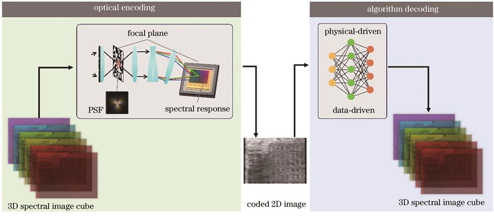
Fig. 1. Main components and operating principle of computational imaging systems
Fig. 2. A discretization example for the spectral image and optical coding
Fig. 3. Optical systems and coding illustrations for single pixel camera. (a) Plain SPC spectral imaging; (b) CHISSS
Fig. 4. Illustration of coded aperture snapshot spectral imagers. (a) DD-CASSI; (b) SD-CASSI
Fig. 5. Illustration of the dual-camera compressive hyperspectral imager
Fig. 6. Illustration for 3D coded aperture imagers. (a) CCA;(b) DCSI; (c) SSCSI
Fig. 7. Example of point spread function encoding system structure
Fig. 8. Representative color filter array and spectral filter array
Fig. 9. Acquisition process of multi-channel images
Fig. 10. Optical systems for spatial duplicating-based encoding. (a) Notch filters have extremely narrow stopband and are able to obtain spectral images with very high spectral resolution in corresponding bands; (b) using FPR arrays with varying thickness to achieve different SRFs, and combining them with lens arrays for spatial replication to capture multi-channel images
Fig. 11. Simple illustrations for architectures of four end-to-end reconstruction neural networks. (a) Simple convolutional neural network; (b) multiscale CNN; (c) generative adversarial network; (d) self-attention operation
| Category | Representative work | Acquisition scheme | Enabling device | Design method |
|---|
| Image plane coding-SPC | Ref.[31],CHISSS[25] | Multiple exposure | DMD,grating | Random coding | | Image plane coding-CASSI | SD-CASSI[13,35],DD-CASSI[34,37] | Direct imaging | Disperser,coded aperture(DMD) | Random coding | | Image plane coding-multiframe coding | Ref.[15,16,38] | Multiple exposure | Disperser,piezo-electric ceramics | Random coding | | Ref.[39] | Multiple exposure | Disperser,piezo-electric ceramics | Optimized coding function | | Ref.[36,28] | Multiple exposure | Disperser,DMD | Random coding | | DCCHI[40-41] | Dual-camera | Splitter,disperser, coded aperture | Random coding | | Image plane coding-3D coding | Ref.[42-43] | Direct imaging | Disperser,CCA | Optimized coding function | | Ref.[28] | Multiple exposure | DMD,filter | Random coding | | DCSI[29] | Multiple exposure | DMD,grating,LCoS | Random coding | | SSCSI[27] | Direct imaging | Grating,coded ape-rture | Random coding | | PSF coding,scattering coding | Ref.[48] | Direct imaging | Scattering medium | Random PSF | | PSF coding-dispersion coding | Ref.[47,50] | Direct imaging | DOE | Random DOE surface | | Ref.[51] | Direct imaging | Disperser | Dispersive PSF | | PSF coding-diffraction coding | Ref.[52-53] | Direct imaging | DOE | Manually designed DOE | | Ref.[46,55] | Direct imaging | DOE | Deeply learned DOE | | SRF coding-fixed SRF | CS-MUSI[76,25,60] | Multiple exposure | Polarizer,liquid crystal | Fixed SRF | | Ref.[65] | Multiple exposure | Liquid crystal,metasurface | | Ref.[69] | Spatially duplicating | Notch filter | | Ref.[61] | Spatially duplicating | FPR array | | SRF coding-random SRF | Ref.[62,77] | Direct imaging | Metasurface | Random SRF | | SRF coding-optimized SRF | Ref.[70] | Direct imaging,Spatially duplicating | Thin film | Deeply learned SRF | | BEST[72-73] | Direct imaging | Metasurface,thin film | | Ref.[75] | Multiple exposure | Thin film | | Ref.[74] | Direct imaging | Superposition FPR | | Image plane coding,SRF coding | SCCSI[26] | Direct imaging | Disperser,CCA-SFA | Random coding | | Ref.[44] | Multiple exposure | LCTF,DMD | Random coding,fixed SRF | | PSF coding,SRF coding | DiffuserCam[49] | Direct imaging | Scattering medium,SFA | Random PSF,fixed SRF |
|
Table 1. Summary of optical encoding methods
| Dataset | Spectrum /nm | Step /nm | Dimension | Size | Camera model | Illumination |
|---|
| CAVE[108] | 400‒700 | 10 | 512×512 | 32 | VariSpec Liquid Crystal Tunable Filter,Apogee Alta U260 | CIE Standard Illuminant D65 | | Harvard[109] | 420‒720 | 10 | 1392×1040 | 75 | Commercial hyperspectral camera with LCTF(Nuance FX,CRI Inc) | Natural Daylight Lighting,Artificial Mixed Lighting | | NUS[104] | 400‒700 | 10 | 1312×950 | 66 | Specim PFD-CL-65-V10E | Natural Light Source,Artificial Broadband Light Sources with Various Color Temperatures | | ICVL[18] | 400‒1000 | 1.25 | 1392×1300 | 200 | Specim PS Kappa DX4,Rotary Stage | Natural Light Source | | 400‒700 | 10 | | KAIST[93] | 420‒720 | 10 | 2704×3376 | 30 | GS3- U3-91S6M-C | Xenon Lamp | | NTIRE2018[110] | 400‒700 | 10 | 1392×1300 | 256 | Specim PS Kappa DX4 | Natural Light Source | | NTIRE2020[106] | 400‒700 | 10 | 482×512 | 460 | Specim IQ | Natural Light Source | | C2H-Data[111] | 374.1‒988.1 | 4.6 | 1392×1650 | 697 | GaiaField System | Tungsten Halogen Lamp | | 450‒740 | 10 | | KAUST-HS[112] | 400‒1000 | 10 | 512×512 | 400 | Specim IQ | Natural Light Source | | NTIRE2022[107] | 400‒700 | 10 | 482×512 | 1000 | Specim IQ | Natural Light Source |
|
Table 2. Summary of popular datasets of spectral images
| Category | Algorithm | Related work | Prior type |
|---|
Sparse approximation | OMP | Ref.[81,18] | | | GPSR | Ref.[13,26,38] | | | TVrestriction | GAP-TV | Ref.[14] | | | TwIST | Ref.[16,36,40] | | | Low rank structure | ADMM | Ref.[88‒89] | | | Tensor decomposition | ADMM | Ref.[91‒92] | Restriction of tensor decomposition | | Learned Prior | ADMM | Ref.[93] | Learned auto-encoder | | SGD | Ref.[94‒95] | Restriction of tensor decomposition,low-dimensional manifold | | Unrolled HQS | Ref.[19,100] | Neural network | | Unrolled ADMM | Ref.[96,98] | Neural network | | Unrolled GAP | Ref.[97] | Neural network |
|
Table 3. Summary of spectral reconstruction algorithms based on physical model and prior knowledge
| Category | Related work | Optical system | Key ingredient |
|---|
| CNN | HSCNN[20] | RGB/CASSI | | | HCSNN+[96] | RGB | Residual connection,dense connection | | HyperReconNet[104] | CASSI | 2D-3D convolution | | BTR-Net[130] | SRF coded | Functional sub-networks | | Wang et al.[62] | SRF coded | Residual connection | Multiscale CNN | Galliani et al.[79] | RGB | Dense connection | | Yan et al.[110] | RGB | Pixel shuffle | | C2H-Net[111] | RGB | Extra class/location information | | DeepCubeNet[104] | SRF coded | | | Baek et al.[46] | PSF coded | | | GAN | Alvarez et al.[97] | RGB | | | R2H-GAN[113] | RGB | Extra spectral discriminator | | Lambda-Net[112] | CASSI | Self attention | Attention-based networks | HRNet[115] | RGB | Dense connection,self attention | | AWAN[116] | RGB | Self attention,SRF-aware | | HDRAN[117] | RGB | 2D-3D self attention,restriction of tensor decomposition | | HD-Net[118] | CASSI | Frequency domain supervision | | TSA-Net[119] | CASSI | Independent 3D attention | | SDNet[120] | SRF coded | Unsupervised training by resampling | | GMSR[121] | RGB | Mamba architecture | | Transformer | MST[122] | CASSI | Coding function-aware | | CST[123] | CASSI | Clustering,coarse-to-fine reconstruction | | ST++[124] | RGB | Coarse-to-fine reconstruction | | TCSSA[125] | RGB | Convolutional spectral self attention |
|
Table 4. Summary of end-to-end spectral reconstruction methods