
Peipei Jiang, Yan Yang. Adaptive Linear Transformation Image Dehazing Algorithm Based on Gaussian Attenuation[J]. Laser & Optoelectronics Progress, 2019, 56(10): 101002
- Laser & Optoelectronics Progress
- Vol. 56, Issue 10, 101002 (2019)

Fig. 1. Flow chart of proposed algorithm
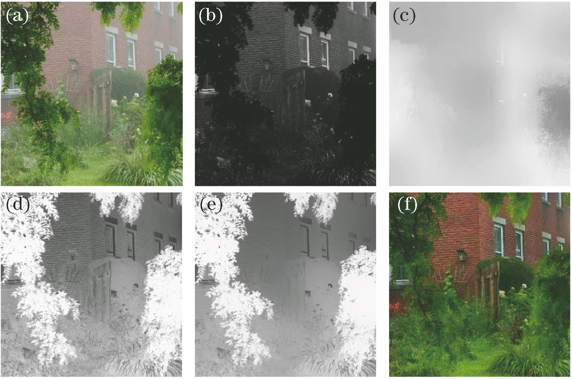
Fig. 2. Effect images of proposed algorithm. (a) Hazy image; (b) adaptive linear transformation; (c) local atmospheric optical value; (d) rough transmittivity; (e) optimal transmittivity; (f) restored image
Fig. 3. Curve of quadratic function
Fig. 4. Comparison of simulation experiments. (a) Hazy image; (b) μ=0.2; (c) μ=0.4; (d) μ=0.6; (e) μ=0.8; (f) μ=1.0
Fig. 5. Comparison of transmittivity. (a) Hazy image; (b) method in Ref. [5]; (c) rough transmittivity; (d) optimal transmittivity
Fig. 6. Effect images based on local atmospheric optical value. (a) Hazy image; (b) map of maximum channel; (c) morphologically closed operation; (d) cross-bilateral filtering result
Fig. 7. Comparison of experimental results. (a) Hazy image; (b) method in Ref. [5]; (c) method in Ref. [6]; (d) method in Ref. [7]; (e) method in Ref. [8]; (f) method in Ref. [9]; (g) proposed method
Fig. 8. Objective evaluation. (a) Number of visible edges; (b) normalized average gradient; (c) number of pixels in saturation point; (d) running time


Set citation alerts for the article
Please enter your email address

© Copyright 2018-2021 | Chinese Laser Press. All Rights Reserved 沪ICP备15018463号-20