Dongqing Huang1,2,3, Weiming Xu1,2,3,*, Wendi Xu1,2,3, Xiaoying He1,2,3, and Kaixiang Pan1,2,3
Author Affiliations
1The Academy of Digital China, Fuzhou University, Fuzhou 350108, Fujian, China2Key Laboratory of Spatial Data Mining & Information Sharing, Ministry of Education, Fuzhou University, Fuzhou 350002, Fujian, China3National Engineering Research Centre of Geospatial Information Technology, Fuzhou University, Fuzhou 350002, Fujian, Chinashow less
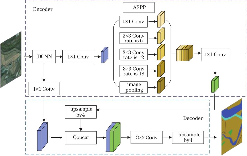
Fig. 1. Network architecture of DeeplabV3+
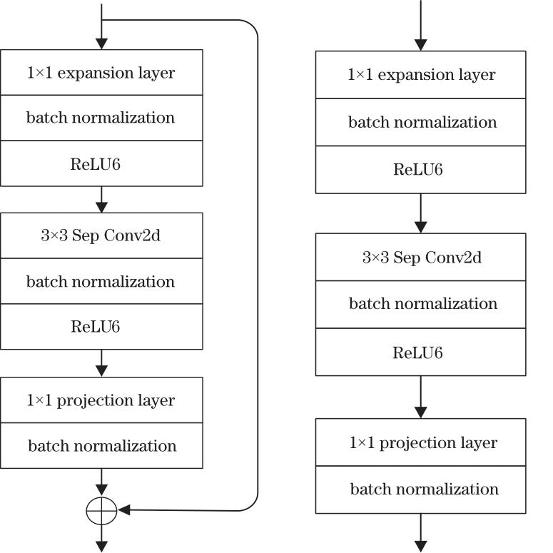
Fig. 2. Bottleneck residual block
Fig. 3. Network architecture of Xception_65
Fig. 4. Network architecture of MS-XDeeplabV3+ and MS-MDeeplabV3+
Fig. 5. Schematic of DCA structure
Fig. 6. Partial samples of CCF dataset
Fig. 7. Comparison of the classification results of the four models. (a) Original image; (b) label; (c) MDeeplabV3+; (d) XDeeplabV3+;(e) MS-MDeeplabV3+; (f) MS-XDeeplabV3+
| Model structure | Encoder | | Decoder |
|---|
| MobilenetV2 | Xception_65 | | Skip a layer fusion | Layer-by-layer fusion | Channel module | Multi-scale supervision |
|---|
| MDeeplabV3+ | √ | | | √ | | | | | XDeeplabV3+ | | √ | | √ | | | | | MS-MDeeplabV3+ | √ | | | | √ | √ | √ | | MS-XDeeplabV3+ | | √ | | | √ | √ | √ |
|
Table 1. Similarities and differences between the four network structures
| Input size | Operation | t | c | n | s |
|---|
| 2562×3 | Conv2d | | 32 | 1 | 2 | | 1282×32 | Bottleneck | 1 | 16 | 1 | 1 | | 1282×16 | Bottleneck | 6 | 24 | 2 | 2 | | 642×24 | Bottleneck | 6 | 32 | 3 | 2 | | 322×32 | Bottleneck | 6 | 64 | 4 | 2 | | 162×64 | Bottleneck | 6 | 96 | 3 | 1 | | 162×96 | Bottleneck | 6 | 160 | 3 | 1 | | 162×160 | Bottleneck | 6 | 320 | 1 | 1 |
|
Table 2. Detailed configuration of the MobilenetV2
| Parameter | Building | Arable | Forest | Water | Road | Grass | Other |
|---|
| Label | 0 | 1 | 2 | 3 | 4 | 5 | 6 | | Percentage /% | 2.79 | 50.87 | 17.87 | 17.74 | 0.35 | 1.96 | 7.38 |
|
Table 3. Proportion of each category in the CCF dataset
| Method | IoU | mIoU | OA | Kappa |
|---|
| Building | Arable | Forest | Water | Road | Grass | Other |
|---|
| MDeeplabV3+ | 0.6882 | 0.8047 | 0.7828 | 0.8249 | 0.2015 | 0.2286 | 0.6233 | 0.5934 | 0.8027 | 0.7735 | | XDeeplabV3+ | 0.7144 | 0.8240 | 0.8267 | 0.8706 | 0.2554 | 0.2034 | 0.6480 | 0.6204 | 0.8348 | 0.7992 | | MS-MDeeplabV3+ | 0.7217 | 0.8234 | 0.8186 | 0.8625 | 0.3431 | 0.2298 | 0.6442 | 0.6348 | 0.8502 | 0.8297 | | MS-XDeeplabV3+ | 0.7650 | 0.8836 | 0.8437 | 0.9168 | 0.4774 | 0.3309 | 0.6615 | 0.6970 | 0.9122 | 0.8646 |
|
Table 4. Quantitative evaluation of the classification results of each model
| Methed | Parameter size /MB | Time /min | mIoU |
|---|
| FCN | 364.7 | 37.8 | 0.5586 | | U-Net | 305.3 | 33.6 | 0.5739 | | SegNet | 307.6 | 34.5 | 0.5748 | | DeeplabV3+ | 312.2 | 39.1 | 0.6199 | | E-Deeplab | 387.3 | 47.8 | 0.6835 | | Algorithm in Ref.[18] | 246.4 | 37.2 | 0.6621 | | Algorithm in Ref.[19] | 332.6 | 42.4 | 0.6537 | | MDeeplabV3+ | 52.7 | 13.3 | 0.5934 | | XDeeplabV3+ | 148.5 | 18.7 | 0.6204 | | MS-MDeeplabV3+ | 55.3 | 17.6 | 0.6348 | | MS-XDeeplabV3+ | 151.1 | 23.9 | 0.6970 |
|
Table 5. Comparison of different network models' training results
| ID | Weight of side output | | mIoU | OA | Kappa |
|---|
| D1 | D2 | D3 | D4 | |
|---|
| 1 | 0 | 0 | 0 | 1 | | 0.6159 | 0.8214 | 0.7975 | | 2 | 0.3 | 0.3 | 0.8 | 1 | | 0.6317 | 0.8485 | 0.8283 | | 3 | 1 | 1 | 1 | 1 | | 0.6348 | 0.8502 | 0.8297 |
|
Table 6. Comparison of different loss weights for
| ID | Weight of side output | | mIoU | OA | Kappa |
|---|
| D1 | D2 | D3 | D4 | |
|---|
| 1 | 0 | 0 | 0 | 1 | | 0.6681 | 0.8827 | 0.8447 | | 2 | 0.3 | 0.3 | 0.8 | 1 | | 0.6933 | 0.9096 | 0.8629 | | 3 | 1 | 1 | 1 | 1 | | 0.6970 | 0.9122 | 0.8646 |
|
Table 7. Comparison of different loss weights for