Coal is an important energy in the world and it plays an important role in the development of the economy. Although a lot of new energy sources are applied in production and living, it will still occupy the dominant position for a long time^[1]. As the demand for coal increases and surface resources decrease, deep mines are concerned and carried out. However, disasters caused by deep mining threaten safety operation seriously. Many methods had been implemented to ensure the operation safety, such as safety pre-evaluation^[2], regional pre-diction^[3], rock mass classification^[4] and so on. Whereas, traditional geological monitoring methods usually require extensive field work, which is time-consuming and labor-intensive. At present, remote sensing has become one of the most effective tools for monitoring the condition of underground spaces. Rock classification based on light detection and ranging (LiDAR) technology attracted wide attention due to its high classification accuracy and good recognition precision^[5].

LiDAR is an effective remote sensing technique that it can not only assess stability of rock conditions accurately^[6], but also collect surface geometry information of rock and distinguish different rock properties by acquiring 3D point cloud data^[7]. Whereas, traditional LiDAR sensors operate at single or several wavelengths that can only obtain limited spectral information, which restrict the performance of application^[8]. With development of remote sensing, the emergence of hyperspectral LiDAR (HSL), fusion of hyperspectral data and LiDAR, significantly enhanced the quantitative and qualitative analysis capabilities of LiDAR, which has been widely used in atmospheric detection, forest protection and artificial target detection^[9-13].

However, the performance of HSL depends on the quality of intensity signal received by LiDAR receiver. Many aspects impact the accuracy of LiDAR intensity signals in on-site applications, such as, instrument properties^[14] and environmental factors^[15]. The common solution is to calibrate the intensity signal to eliminate data deviation. In 2007, Hoefle et al. calibrated the intensity signal using data-driven and model-driven correction, which provided support for surface classification and multi-temporal analysis^[16]. In 2011, Kaasalainen et al. studied the effect of range and incidence angle on intensity signals, conducted instrument calibration and target surface features calibration researches^[14]. In the same year, Yan et al. evaluated the influence of geometric calibration and radiometric calibration of LiDAR signal on land surface classification, improved the accuracy of LiDAR data by eliminating parameter deviations and correcting the scanning angle^[17]. Most calibration methods need a whiteboard with a calculated reflectance as reference to correct LiDAR signals. While the environment of signal collection site is seriously polluted and the reference whiteboard is easily covered by dust, which leads to inaccurate calculations and is hard to ensure the accuracy of calibration.

To address this issue, we propose a new method to classify coal/rock samples without calibration. The instrument we employed is previously proposed an HSL based on acousto-optic tunable filter (AOTF)^[18], which offers a quicker tuning speed and broader wavelength ranges. First, waveform entropy (WE) and joint skewness-kurtosis figure (JSKF) are calculated based on HSL intensity signals, as new extracted features. Then, coal/rock samples are classified with WE and JSKF by random forest (RF) and support vector machine (SVM) classifiers and the classification results are compared with the intensity signals. Finally, with spectral segmentation test, the classification performances are optimized by selecting the fewer channels and compared results with calibrated intensity signal.

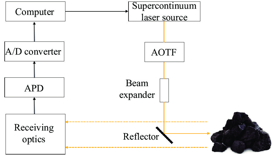
The instrument we employed is the previously designed AOTF-HSL with a spectral 5 nm resolution, using a supercontinuum laser source (YSL® SC-OEM)^[18], as Fig.1 shown. A computer triggers laser source to transmit supercontinuum laser pulses and filtered by the AOTF device to select specific wavelength. The specifications of AOTF module can be found in Tab.1. With beam expander, the laser pulses are collimated to transmit to the target. The echo signals are collected by the optical receiving module and focused them on avalanche photodiode (APD) model, which converts the laser echo signals into electronic signals and amplifies them. The output signals of APD are sampled and converted to digital signals by a high-speed A/D converter and transmitted to computer for data processing.

The measurements were conducted in a controlled laboratory environment to obtain hyperspectral information through AOTF-HSL. Due to the low sensitivity of APD and the low transmitted power intensity of supercontinuum lasers below 650 nm^[19], the measurement of the spectrum channels was selected in the range of 650 nm to 1100 nm. The waveforms of pulses reflected from coal/rock samples were collected by an oscilloscope sampling at 20 GHz.

Besides coal and gangue-rock, we also added rock from roof layer and rock from floor layer as samples, which come from deep mines^[18]. All samples were scanned at the same distance from the instrument that range differences between samples can be neglectable.

The precision of the intensity calibration of HSL system is a prerequisite for many quantitative applications, and it has become an important research object^[14]. The equation (1) describes parameters related to the signal received by the LiDAR sensor:

$ {P}_{\rm r}=\frac{{P}_{\rm t}{D}_{\rm r}^{2}}{4\pi {R}^{4}{\beta }_{\rm t}^{2}}\sigma $ (1)

Where, P_r is the power receiver, P_t is the transmitted power, D_r is the receiver optical aperture diameter, R is the distance, β_t denotes transmitter beam width, and σ is the backscatter cross section.

The backscatter cross section can be expressed equation (2):

$ \sigma =\frac{4\pi }{\varOmega }\rho {A}_{S} $ (2)

Where, Ω is a cone of a solid angle into which the incoming radiation is scattered uniformly, ρ is the surface reflectance, and A_S denotes the scattering receiving area.

The equations indicate that the accuracy of intensity signals not only depends on distance, scattering cross-section, and atmospheric parameters, but also relates to reflectance of targets and directionality of the incident angle^[15]. Therefore, it is necessary to calibrate intensity signals. An efficient calibration method is to set a whiteboard with a constant reflectance for correction^[18]. Whereas, in deep coal mines, the conventional calibration method is hard to valid because of dust pollution.

The entropy concept is introduced to measure uncertainty of random variables^[20]. A metric of the dispersion degree of echo signals with respect to their variables is selected as a new feature, namely waveform entropy.

While the different target is present, the entropy value corresponds different, further, WE parameter of the same target is different under different spectral laser scanning^[21]. Therefore, we can distinguish different type sequences based on WE, which is vary with scatter distribution, wavelength and other features^[21-22].

In order to adopt the concept of entropy, we suppose digital echo signals as X_j^t= x_j^t(i), i= n,···,N, t=1,···4, j=1,···m. i denotes the echo signal from initial point to the ending point, t is the different type of coal sample, and j is the number of channels, setting,

$ {X}_{j}^{t}=\sum\limits _{i=n}^{N}\left|{x}_{j}^{t}\left(i\right)\right| $ (3)

$ {p}_{j}^{t}\left(i\right)=\frac{{\left|{x}_{j}^{t}\left(i\right)\right|}^{2}}{{\left({X}_{j}^{t}\right)}^{2}} $ (4)

Where, p_j^t(i) is an energy distribution of the vector at individual components, WE is defined as,

$ {E}_{j}^{t}\left(x\right)=-\sum\limits _{i=n}^{N}{p}_{j}^{t}\left(i\right)\mathit{\rm ln}{p}_{j}^{t}\left(i\right) $ (5)

Evidently, WE is closely related with amplitude, and vary with signal amplitude fluctuation. The more uniform probability p_j^t(i) is, the larger WE value is. Consequently, WE of a digital waveform depends on the waveform itself, we will apply the distinguished values as feature to classify the different coal samples.

Digital waveform provides more specific information potentially which easily available for operation^[23]. Statistical variables of waveform energy were extracted from LiDAR echo signal waveform, which has been widely applied in the discriminated classes of coastal habitats and species^[24], forest species^[25]. In 2011, Guo et al.^[26] proposed a JSKF model by combining skewness and kurtosis for band selection and achieved good results. We employ JSKF as a new feature to classify coal/rock.

Skewness is a characteristic number that characterizes the degree of asymmetry of the probability distribution density curve relative to the average, which is expressed by the third-order standardized moments. The equation is:

$ S=\frac{E{[X-\mu ]}^{3}}{{\sigma }^{3}} $ (6)

Where, E(X) is the expectation of vector X, μ is the mean value of vector X, and σ is the standard deviation of vector X. The larger the skewness, the more asymmetrical the distribution of random variables.

Kurtosis is a characteristic number that characterizes the peak of the probability density distribution curve at average value, which is expressed by the ratio of the fourth-order central moment of the random variable to the square of the variance. Kurtosis reflects the sharpness of the peak of the probability density distribution curve. The larger the kurtosis value, the sharper the probability density distribution curve. The equation is:

$K=\frac{E{[X-\mu ]}^{4}}{{\sigma }^{4}}-3 $ (7)

Skewness and kurtosis represent the asymmetry of random distribution, which could not only measure the difference between different bands of target characteristics, but also evaluate non-Gaussianity of data samples. JSKF uses the product of skewness and kurtosis as an indicator to measure the amount of information deviating from the normal distribution of the size. It is defined as

$ {F}_{\rm JSKF}=S\cdot K $ (8)

That is:

$ {F}_{\rm JSKF}=\frac{1}{{\sigma }^{7}}\left[E{\left(X-\mu \right)}^{4}-3{\sigma }^{4}\right]\cdot E{(X-\mu )}^{3} $ (9)

It is obvious that JSKF is related to the expectation of the waveform. The expectation is related to mean and standard deviation. The mean and standard deviation depend on the waveform itself. Therefore, the JSKF of the digital waveform also depends on the waveform itself that has no relation to external conditions. We employ the waveform of JSKF as another feature to classify different coal and rock samples in the next section.

In order to explore coal/rock classification based on AOTF-HSL, RF and SVM are employed as classifiers in our experiments. The main advantage of RF is only a few parameters and manual intervention needed to require high stability^[27], which is usually applied for remote sensing image analysis^[28]. SVM can provide high classification accuracy and it has become a very popular kernel-based classification algorithm in hyperspectral image classification^[29]. Both of them have been widely applied in remote sensing researches and their efficiencies have proven in remote sensing data classification^[30]. Multi-label classification is implemented by the scikit-learn Python package^[31].

The experiments were conducted under a controlled laboratory environment. We employed HSL of 91 channels to collect different coal/rock sample data and calculated WE and JSKF based on echo signals. Then, intensity signals, WE, JSKF, and calibrated intensity signals were classified by RF and SVM classifiers to observe the performance.

With the number of channels in HSL increases, the instrument complexity and the amount of collected data also increase at the same time. Complex large-scale instruments and huge data volumes are hard for on-site operation and data processing. Therefore, we hope that a miniaturization HSL with less channels can also achieve accurate classification results. In order to simplify equipment complexity to save equipment resources and improve efficiency, we have improved the experiment: select a part of channels from 91 channels for classi-fication by random selection method and test accuracy. The number of channels increases from 1 in turn until the precision reaches 100%. We evaluate the consequences by comparing the number of channels required.

To further compare the capacity of WE, JSKF and calibrated intensity signals, we attempt to randomly extract 5 channels from 91 channels and assess the property of them respectively. At the same time, our previous research confirmed that the data of different bands have different properties^[32], so we conduct a spectral segmentation test based on WE and JSKF to find the optimal band for classification.

The classification results of all channels are shown in the Tab.2. The accuracy of all features can reach 100% by using the full channels spectral information. The results prove that with sufficient spectral information, the classification of coal and rock can achieve ideal results.

With sufficient experiment tests, the channels of random selected classification results are shown in the Tab.3. For the RF classifier, while accuracy reaches 100%, the least number of channels needed for intensity signal is 21, which is maximum compared with others. WE needs 15 channels, the channels of JSKF and calibrated intensity signal are both 6. Compared with the intensity signal, WE, JSKF and calibrated intensity signal reduce 6, 15, 15 channels respectively. For the SVM classifier, when accuracy reaches 100%, the intensity signal needs 20 channels at least. WE needs 15 channels, JSKF needs 6 channels, and the calibrated intensity signal needs 4 channels. Compared with the intensity signal, WE, JSKF and calibrated intensity signal reduce 5, 14, 16 channels respectively. With comparison, we can draw a conclusion: the four groups of data can still achieve the desired performances by using fewer spectrum channels. Meanwhile, the number of channels needed for WE and JSKF classification is significantly less than that of intensity signal. Although WE and JSKF do not achieve the classification ability as same as calibrated intensity signal, they can provide enhancement of classification effect significantly than the intensity signal, which indicate that the HSL intensity signal calibration-free method we proposed is feasible for improving the classification performance.

5-channel random extraction classification results are shown in Tab.4. The accuracies are calculated by averaging multiple experiments.

From the results, we can see that with 5 channels, the accuracy of calibrated intensity signal and JSKF is 98% and 96% respectively by RF, and they are both 100% by SVM. For WE, although more channels are needed to achieve accurate classification, the precision still reaches 90% by extracting 5 channels randomly. The reason is that the 91-channel HSL covers a wide spectrum that different spectral bands have different classification properties^[32]. Therefore, we conduct a spectrum segmentation test to find the optimal interval of classification.

Figure 2 show the waveform distribution diagram of WE and JSKF.

We can see that WE and JSKF present different properties in different bands. For WE, the entropy changes slowly at 650-1000 nm and increases significantly at 1000-1100 nm in Fig.2(a). JSKF is used as an indicator to measure the amount of information that deviates from the normal distribution. The data are approximately at the lowest value between 720 nm and 820 nm in Fig.2(b). That means, the data deviation is relatively low; and when it reaches the maximum at 1000-1100 nm, the data deviation is relatively high. Thus, we test the 720-820 nm band and the 1000-1100 nm band respectively and compared them with the calibrated intensity signal. There are 20 channels in each band. The results are shown in Tab.5 and Tab.6.

From Tab.5, we can see that in the 720-820 nm spectrum band, for the WE, the precision is only reach 95% using all of 20 channels, whereas the performance of JSKF is improved further compared to random channels selection method. The 100% accuracy only needs 3 channels with RF classifier, and needs 6 channels with random channels selection. And the 100% accuracy only needs 4 channels with SVM classifier, where efficiency increased 33% than random channels selection. In this band, the number of channels that accuracy reach 100% needed for JSKF is basically as same as the number of channels required for calibrated intensity signal.

From Tab.6, we can see that in the 1 000 - 1 100 nm spectrum band, the performance of WE has been improved further than random channel selection method. The 100% accuracy only needs 11 channels with RF classifier, and increase 27% than channel selection randomly, and it needs 7 channels with SVM classifier, which improve 53% than channel selection randomly. For JSKF, the performance is slightly reduced. The number of channels of RF and SVM classifiers is reduced by 217% and 40% compared with random channel selection. In this band, the number of channels needs to reach 100% accuracy with WE is basically as same as the number of channels required with calibrated intensity signal.

Based on the above experiments, we can see that WE and JSKF have different classification results in different spectral band. The reason is as following: WE characterizes the degree of dispersion for variables. Due to the different characteristic wavelength of object, the absorption characteristic of the spectrum is different. The characteristic wavelength of coal/rock is in the near-infrared spectrum^[33], where the absorption characteristic is obvious, the degree of dispersion for variables is large and WE changes significantly (Fig.2(a)). Thus, the classification performance of WE is better in the near-infrared band. JSKF measures the deviation of the variable from the normal distribution. The smaller the data deviation, the better the data quality. The data collection results show that the deviation of the data is small in 720-820 nm band (Fig.2(b)). Thus, the classification performance of JSKF is better in 720-820 nm band. Meanwhile, both of them can basically reach the classification performance of calibrated intensity signal in their corresponding ideal classification band. While realizing the intensity signal calibration-free, it maintains excellent classification performances. The results show that our calibration-free classification method is feasible.

In this paper, we proposed a new method based on the classification of coal/rock in deep coal mines. Without any reference, we employed WE and JSKF to classify four different types of coal/rock, explored the classification performances of different features in different spectral bands and evaluated the classification performance by comparing with calibrated intensity signal. The following conclusions can be drawn from the results:

(1) When the spectral information is sufficient, all features can achieve accurate classification.

(2) WE and JSKF require less spectral channels than intensity signals to achieve accurate classification.

(3) For different spectral bands, WE and JSKF have different classification performance, and they can achieve great classification performance as calibrated intensity signal in their ideal band.

This research not only solves the problem that intensity signals cannot be calibrated in the deep coal mines, but also simplify the complexity of the equipment, laying the foundation for miniaturized LiDAR. In the future, we will do the further research for instrument miniaturization package and deep mine field application.

References

[1] Feng Qun, Chen Hong. The safety-level gap between China and the US in view of the interaction between coal production and safety management. Safety Science, 54, 80-86(2013).
[2] Qingjie Qi, Xiaoliang Zhao, Baichao Song. Pre-evaluation method of coal mine safety based on continental distance model with varying weight. Procedia Earth and Planetary Science, 1, 180-185(2009).
[3] Weihua Song, Hongwei Zhang. Regional prediction of coal and gas outburst hazard based on multi-factor pattern recognition. Procedia Earth and Planetary Science, 1, 347-353(2009).
[4] V M Khatik, A K Nandi. A generic method for rock mass classification. Journal of Rock Mechanics and Geotechnical Engineering, 10, 106-120(2018).
[5] L Weidner, G Walton, R A Kromer. Classification methods for point clouds in rock slope monitoring: A novel machine learning approach and comparative analysis. Engineering Geology, 263, 105326(2019).
[6] A K Ryan, Jean H D, M J Lato, et al. Identifying rock slope failure precursors using LiDAR for transportation corridor hazard management. Engineering Geology, 195, 93-103(2015).
[7] P Hartzell, C Glennie, K Biber, et al. Application of multispectral LiDAR to automated virtual outcrop geology. ISPRS Journal of Photogrammetry and Remote Sensing, 88, 147-155(2014).
[8] Yuwei Chen, Changhui Jiang, Juha Hyyppa, et al. Feasibility study of ore classification using active hyperspectral LiDAR. IEEE Geoscience and Remote Sensing Letters, 15, 1785-1789(2018).
[9] Bingyi Liu, Quanfeng Zhuang, Shengguang Qin, et al. Aerosol classification method based on high spectral resolution lidar. Infrared and Laser Engineering, 46, 0411001(2017).
[10] Junfa Dong, Jiqiao Liu, Xiaolei Zhu, et al. Splitting ratio optimization of spaceborne high spectral resolution lidar. Infrared and Laser Engineering, 48, S205001(2019).
[11] Junjie Xu, Lingbing Bu, Jiqiao Liu, et al. Airborne high-spectral-resolution lidar for atmospheric aerosol detection. Chinese Journal of Lasers, 47, 0710003(2020).
[12] Morsdorf, Nichol, Malthus, et al. Assessing forest structural and physiological information content of multi-spectral LiDAR waveforms by radiative transfer modelling. Remote Sensing of Environment, 113, 2152-2163(2009).
[13] Yuwei Chen, E Räikkönen, S Kaasalainen, et al. Two-channel hyperspectral LiDAR with a supercontinuum laser source. Sensors, 10, 7057-7066(2010).
[14] K Sanna, J Anttoni, K Mikko, et al. Analysis of incidence angle and distance effects on terrestrial laser scanner intensity: search for correction methods. Remote Sensing, 3, 2207-2221(2011).
[15] M A F Balduzzi, V D Z Dimitry, J Stuckens, et al. The properties of terrestrial laser system intensity for measuring leaf geometries: A case study with conference pear trees (Pyrus Communis). Sensors, 11, 1657-1681(2011).
[16] B Hoefle, N Pfeifer. Correction of laser scanning intensity data: Data and model-driven approaches. ISPRS Journal of Photogrammetry and Remote Sensing, 62, 415-433(2007).
[17] W Y Yan, A Shaker, A Habib, et al. Improving classification accuracy of airborne LiDAR intensity data by geometric calibration and radiometric correction. ISPRS Journal of Photogrammetry and Remote Sensing, 67, 35-44(2012).
[18] Hui Shao, Yuwei Chen, Zhirong Yang, et al. A 91-channel hyperspectral LiDAR for coal/rock classification. IEEE Geoscience and Remote Sensing Letters, 17, 1052-1056(2020).
[19] Yuwei Chen, Wei Li, H Juha, et al. A 10-nm spectral resolution hyperspectral LiDAR system based on an acousto-optic tunable filter. Sensors, 19, 1620(2019).
[20] R CoifmanR, M V Wickerhauser. Entropy-based algorithms for best basis selection. IEEE Transactions on Information Theory, 38, 713-718(1992).
[21] D J Diner, F Xu, J GarayM, et al. The Airborne Multiangle Spectro Polarimetric Imager (AirMSPI): A new tool for aerosol and cloud remote sensing. Atmospheric Measurement Techniques, 6, 2007-2025(2013).
[22] Jikai Chen, Guoqing Li. Tsallis wavelet entropy and its application in power signal analysis. Entropy, 16, 3009-3025(2014).
[23] A Hovi, L Korhonen, J Vauhkonen, et al. LiDAR waveform features for tree species classification and their sensitivity to tree- and acquisition related parameters. Remote Sensing of Environment, 173, 224-237(2016).
[24] Dianpeng Su, Fanlin Yang, Yue Ma, et al. Classification of coral reefs in the south China sea by combining airborne LiDAR bathymetry bottom waveforms and bathymetric features. IEEE Transactions on Geoscience and Remote Sensing, 57, 815-828(2019).
[25] Zhujun Gu, Sen Cao, G A Sanchez-Azofeifa. Using LiDAR waveform metrics to describe and identify successional stages of tropical dry forests. ITC Journal, 73, 482-492(2018).
[26] Lei Guo, Weiwei Chang, Chaoyang Fu. Band selection of optimal for hyperspectral image fusion. Journal of Astronautics, 32, 374-379(2011).
[27] C W Chan, P Desiré. Evaluation of random forest and adaboost tree-based ensemble classification and spectral band selection for ecotope mapping using airborne hyperspectral imagery. Remote Sensing of Environment, 112, 2999-3011(2008).
[28] N Ghasemian, M Akhoondzadeh. Introducing two Random Forest based methods for cloud detection in remote sensing images. Advances in Space Research, 62, 288-303(2018).
[29] Chunhui Zhao, Bing Gao, Lejun Zhang, et al. Classification of hyperspectral imagery based on spectral gradient, SVM and spatial random forest. Infrared Physics and Technology, 95, 61-69(2018).
[30] I V Emma, Z M Raúl. An evaluation of guided regularized random forest for classification and regression tasks in remote sensing. International Journal of Applied Earth Observations and Geoinformation, 88, 102051(2020).
[31] F Pedregosa, G Varoquaux, A Gramfort, et al. Scikit-learn: Machine learning in python. Journal of Machine Learning Research, 12, 2825-2830(2011).
[32] Hui Shao, Yuwei Chen, Wei Li, et al. An investigation of spectral band selection for hyperspectral LiDAR technique. Electronics, 9, 148(2020).
[33] Shouxun Yan, Bing Zhang, Yongchao Zhao, et al. Summarizing the VIS-NIR spectra of minerals and rocks. Remote Sensing Technology and Application, 18, 191-201(2003).
Set citation alerts for the article
Please enter your email address
© Copyright 2018-2021 | Chinese Laser Press. All Rights Reserved 沪ICP备15018463号-20