
Jianpeng Gao, Liang Sheng, Xinyi Wang, Yanhong Zhang, Liang Li, Baojun Duan, Mei Zhang, Yang Li, Dongwei Hei. Five-view three-dimensional reconstruction for ultrafast dynamic imaging of pulsed radiation sources[J]. Matter and Radiation at Extremes, 2024, 9(2): 027801
- Matter and Radiation at Extremes
- Vol. 9, Issue 2, 027801 (2024)
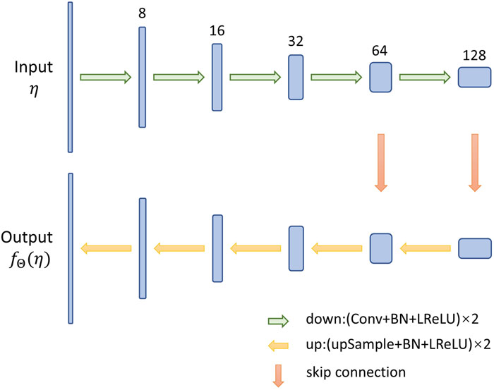
Fig. 1. Structure of neural network.

Fig. 2. The angular distribution of the imaging axes: 1, (90°,180°); 2, (90°,135°); 3, (90°,90°); 4, (90°,45°); 5, (90°,22.5°).
Fig. 3. 3D reconstructed results of three different algorithms. (a1)–(a3) Perspective view, 3D view and slice image at x = 0 of simulated data, respectively. (b1)–(b3) Results of analytical method. (c1)–(c3) Results of iterative method. (d1)–(d3) Results of DIP processing.
Fig. 4. 3D reconstructed results of three different algorithms with noisy data. (a1)–(a3) Perspective view, 3D view, and slice image at x = 0 of analytical results, respectively. (b1)–(b3) Results of iterative method. (c1)–(c3) Results of DIP processing.
Fig. 5. Comparison between projections of reconstruction results and simulation data projections. (a1) Projection of simulation data at angle 1. (a2) Projection with noise. (b1) and (b2) Difference images between simulation data projection and projection of analytical results with and without noisy data. (c1) and (c2) Difference projection images of iterative results with and without noisy data. (d1) and (d2) Difference projection images of iteration with DIP results with and without noisy data.
Fig. 6. Convergence curve of iterative process (a) and loss curve of DIP (b) with and without noisy data.
Fig. 7. Schematic of XUV/SR pinhole imaging system.6
Fig. 8. (a) Raw projection data and (b)–(e) preprocessed images of angle 1 from shot 2 023 052 405.
Fig. 9. 3D spatial distributions of XUV/SR emission reconstructed by analytical method. (a1)–(a4) Reconstructed 3D images from shot 2 023 052 405 at T 1, …, T 4, respectively. (b1)–(b4) Perspective images from shot 2 023 052 405 at T 1, …, T 4, respectively. (c1)–(c4) Reconstructed 3D images from shot 2 023 052 406 at T 1, …, T 4, respectively. (d1)–(d4) Perspective images from shot 2 023 052 406 at T 1, …, T 4, respectively.
Fig. 10. 3D spatial distributions of XUV/SR emission reconstructed by the iterative method with DIP. (a1)–(a4) Reconstructed 3D images from shot 2 023 052 405 at T 1, …, T 4, respectively. (b1)–(b4) Perspective images from shot 2 023 052 405 at T 1, …, T 4, respectively. (c1)–(c4) Reconstructed 3D images from shot 2 023 052 406 at T 1, …, T 4, respectively. (d1)–(d4) Perspective images from shot 2 023 052 406 at T 1, …, T 4, respectively.
Fig. 11. Slice images of XUV/SR emission reconstructed by the iterative method with DIP. (a1)–(a4) XUV/SR emission slice images at z = −47 from shot 2 023 052 405 at T 1, …, T 4, respectively. (b1)–(b4) XUV/SR emission slice images at z = 113 from shot 2 023 052 405 at T 1, …, T 4, respectively.
|
Table 1. Iterative method using cylindrical harmonic decomposition.
|
Table 1. Image assessment indices of sources reconstructed by the analytical method (AM), the iterative method (IM), and iteration with DIP (IM+DIP). Boldface denotes that the image assessment index of corresponding algorithm is better than that of other algorithms.
|
Table 2. Artifact reduction via deep image prior.


Set citation alerts for the article
Please enter your email address

© Copyright 2018-2021 | Chinese Laser Press. All Rights Reserved 沪ICP备15018463号-20