• Photonics Research
  • Vol. 12, Issue 10, 2409 (2024)
Jiahao Dong1, Liang Xu1,6,*, Yiqi Fang2, Hongcheng Ni3..., Feng He4,5, Songlin Zhuang1 and Yi Liu1,5,7,*|Show fewer author(s)
Author Affiliations
  • 1Shanghai Key Laboratory of Modern Optical System, University of Shanghai for Science and Technology, Shanghai 200093, China
  • 2Fachbereich Physik, Universität Konstanz, 78464 Konstanz, Germany
  • 3State Key Laboratory of Precision Spectroscopy, East China Normal University, Shanghai 200241, China
  • 4Key Laboratory for Laser Plasmas (Ministry of Education) and School of Physics and Astronomy, Shanghai Jiao Tong University, Shanghai 200240, China
  • 5CAS Center for Excellence in Ultra-intense Laser Science, Shanghai 201800, China
  • 6e-mail: liangxu2021@usst.edu.cn
  • 7e-mail: yi.liu@usst.edu.cn
  • show less
    DOI: 10.1364/PRJ.528051 Cite this Article Set citation alerts
    Jiahao Dong, Liang Xu, Yiqi Fang, Hongcheng Ni, Feng He, Songlin Zhuang, Yi Liu, "Scheme for generation of spatiotemporal optical vortex attosecond pulse trains," Photonics Res. 12, 2409 (2024) Copy Citation Text show less
    Sketch of the discrete spatial electric dipole approximation. A STOV pumping pulse irradiates a blob of hydrogen atoms, and atoms at different X positions experience different phase and intensity of the driving field, then generating STOV high harmonics. (X,Y,Z) denotes the space coordinate system. (x,y,z) is the local atomic coordinate system, whose origin is located at (X,Y=0,Z=0).
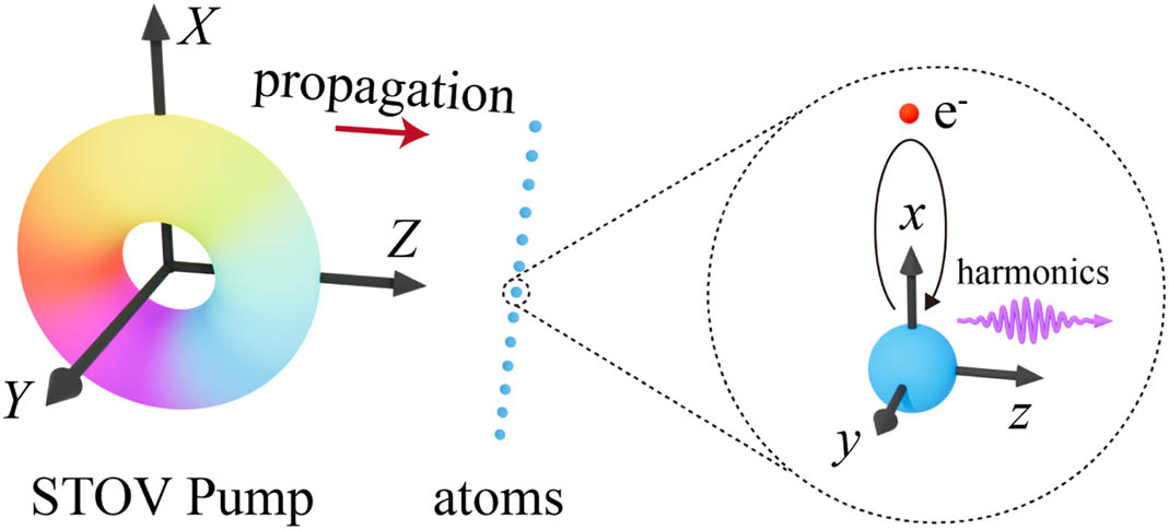
    Fig. 1. Sketch of the discrete spatial electric dipole approximation. A STOV pumping pulse irradiates a blob of hydrogen atoms, and atoms at different X positions experience different phase and intensity of the driving field, then generating STOV high harmonics. (X,Y,Z) denotes the space coordinate system. (x,y,z) is the local atomic coordinate system, whose origin is located at (X,Y=0,Z=0).
    (1st column) Spatial-resolved HHG spectra driven by STOV pulses and retrieved spatiotemporal (2nd column) intensity and (3rd column) phase distributions of the 35th harmonic. (a) Only FW field with λFW=1600 nm; two-color STOV pulses with the phase difference (b) ϕ=0 and (c) ϕ=1.1π between FW and TH fields, respectively. The FW intensity is fixed as IFW=1×10¹⁴ W/cm2, and the TH intensity is ITH=9×10¹² W/cm2. The black dashed line represents the ionization potential of H atom. o.c. is the FW period throughout.
    Fig. 2. (1st column) Spatial-resolved HHG spectra driven by STOV pulses and retrieved spatiotemporal (2nd column) intensity and (3rd column) phase distributions of the 35th harmonic. (a) Only FW field with λFW=1600  nm; two-color STOV pulses with the phase difference (b) ϕ=0 and (c) ϕ=1.1π between FW and TH fields, respectively. The FW intensity is fixed as IFW=1×10¹⁴  W/cm2, and the TH intensity is ITH=9×10¹²  W/cm2. The black dashed line represents the ionization potential of H atom. o.c. is the FW period throughout.
    Diagrams of the time-frequency analyses of the HHG emission (X=0) generated by (a) single STOV pulse and (b), (c) two-color STOV pulses. (a)–(c) correspond to Figs. 2(a1)–2(c1), respectively.
    Fig. 3. Diagrams of the time-frequency analyses of the HHG emission (X=0) generated by (a) single STOV pulse and (b), (c) two-color STOV pulses. (a)–(c) correspond to Figs. 2(a1)–2(c1), respectively.
    Classical electron trajectories driven by laser fields at X=0. (a)–(c) correspond to Figs. 2(a1)–2(c1), respectively. The blue, green, yellow, and red curves represent an electron trajectory with one, two, three, and four or more returns, respectively. The line thickness represents the relative magnitude of the ionization rate after logarithmic treatment. Note that only trajectories where electrons are able to return and the ionization rate is greater than 10% of the maximum ionization rate are shown, and about half of the laser field is shown by the black dashed line.
    Fig. 4. Classical electron trajectories driven by laser fields at X=0. (a)–(c) correspond to Figs. 2(a1)–2(c1), respectively. The blue, green, yellow, and red curves represent an electron trajectory with one, two, three, and four or more returns, respectively. The line thickness represents the relative magnitude of the ionization rate after logarithmic treatment. Note that only trajectories where electrons are able to return and the ionization rate is greater than 10% of the maximum ionization rate are shown, and about half of the laser field is shown by the black dashed line.
    Retrieved spatiotemporal intensity distributions of APT in (a), (b), and (c) correspond to Figs. 2(a1), 2(b1), and 2(c1), respectively. (d) Temporal intensity profiles of a single attosecond pulse sampled from the black rectangle in (c). The red dotted curve represents a Gaussian fitting with an FWHM of 613 as.
    Fig. 5. Retrieved spatiotemporal intensity distributions of APT in (a), (b), and (c) correspond to Figs. 2(a1), 2(b1), and 2(c1), respectively. (d) Temporal intensity profiles of a single attosecond pulse sampled from the black rectangle in (c). The red dotted curve represents a Gaussian fitting with an FWHM of 613 as.
    Spatially-resolved 35th harmonic spectra, ITH=9×10¹² W/cm2 for (a1) and ITH=4.9×10¹³ W/cm2 for (a2). (b) Time-dependent ionization probability for (a) calculated via TDSE. (c1) and (c2) are reconstructed HHG spectra by the quantum-orbit model. The intensity ratios ITH/IFW are taken to be 0.09 and 0.49, respectively. IFW=1×10¹⁴ W/cm2 is fixed in all panels. The X=0 position is considered in (b) and (c).
    Fig. 6. Spatially-resolved 35th harmonic spectra, ITH=9×10¹²  W/cm2 for (a1) and ITH=4.9×10¹³  W/cm2 for (a2). (b) Time-dependent ionization probability for (a) calculated via TDSE. (c1) and (c2) are reconstructed HHG spectra by the quantum-orbit model. The intensity ratios ITH/IFW are taken to be 0.09 and 0.49, respectively. IFW=1×10¹⁴  W/cm2 is fixed in all panels. The X=0 position is considered in (b) and (c).
    Distribution of cos(2ωt−2φf) in the X–t plane, where φf is the azimuthal angle in the space-time plane.
    Fig. 7. Distribution of cos(2ωt2φf) in the Xt plane, where φf is the azimuthal angle in the space-time plane.
    Jiahao Dong, Liang Xu, Yiqi Fang, Hongcheng Ni, Feng He, Songlin Zhuang, Yi Liu, "Scheme for generation of spatiotemporal optical vortex attosecond pulse trains," Photonics Res. 12, 2409 (2024)
    Download Citation