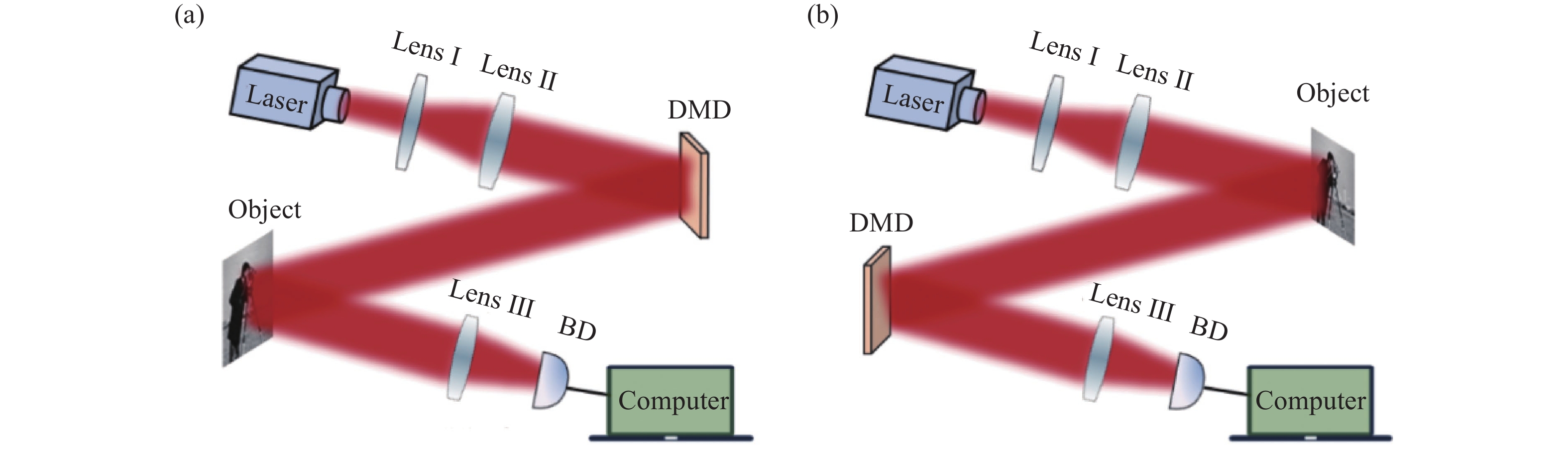
Fig. 1. Schematic diagram of the SPI. (a) The active SPI; (b) The passive SPI

Fig. 2. Schematic diagram of the synthesis and decomposition of 2D image based on Fourier forward and inverse transforms ^[37]

Fig. 3. Schematic diagram of the FSPI experimental system ^[38−39]

Fig. 4. (a) The temporal dithering strategy; (b) The spatial dithering strategy; (c) The reconstructed Fourier spectra and images using different binarization methods^[40]

Fig. 5. (a) The temporal dithering strategy; (b) The signal dithering strategy; (c) The reconstructed images under different spectral coverage^[41]

Fig. 6. (a) Error diffusion kernels of Floyd-Steinberg and Zhang-Qi; (b) Eight different image dithering scanning strategies; (c) Different scanning methods (top row) and corresponding partial amplification (bottom row) based on Zhang-Qi dithering strategies; (d) The experimental results of 3D target scene^[42]

Fig. 7. (a) Schematic diagram based on Gaussian random sampling ^[44]; (b) The reconstruction results at different DMD refresh rates ^[44]; (c) Schematic diagram based on sparse sampling ^[45]; (d) The reconstruction results under different sampling methods ^[45]

Fig. 8. (a) Flowchart of adaptive FSPI based on Fourier domain radial correlation ^[49]; (b) Schematic diagram of the adaptive FSPI based on DQN ^[50]; (c) Adaptive FSPI scheme based on the AuSamNet ^[51]

Fig. 9. (a) Schematic diagram of multi-block FSPI via frequency division multiplexed modulation ^[52]; (b) The reconstruction results of the target at a sampling rate of 1% under different signal-to-noise ratios ^[52]; (c) Schematic diagram of SPI for high performance based on optimized sinusoidal patterns ^[54]; (d) The reconstruction results of the target at a sampling rate of 20% under different signal-to-noise ratios ^[54]

Fig. 10. (a) Representation of nonlocal 3D sparsity in the transform domain; (b) The reconstruction results of different algorithms; (c) The experimental reconstruction results under different sampling rates^[55]

Fig. 11. (a) The generative adversarial network architecture ^[59]; (b) Comparison of reconstruction results under different methods ^[59]; (c) Schematic diagram of high-resolution iterative reconstruction based on diffusion model ^[60]; (d) Comparison of reconstruction methods under different sampling rates ^[60]

Fig. 12. (a) Schematic diagram of dual-contour data processing based on the FSPI ^[67]; (b) Edge detection method based on the FSPI ^[76]

Fig. 13. ^[77] (a) Schematic diagram of polarized computational ghost imaging in scattering system with half-cyclic sinusoidal patterns; (b) The reconstruction results of different methods in the same scattering system

Table 1. Comparison of three different dithering strategies

Table 2. Comparison of different sampling-path strategies

Table 3. Comparison of different reconstruction algorithms