Photoacoustic (PA) imaging (PAI), as a novel non-invasive imaging modality, allows optical imaging of tissues at centimeter-scale depths with acoustic resolution, leveraging contrast based on the optical absorption of tissue components [1,2]. Photoacoustic imaging can be broadly categorized into photoacoustic microscopy (PAM) and photoacoustic tomography (PAT). PAT has gained widespread application in in-vivo imaging due to its distinctive advantages in imaging field of view (FOV) and depth [3,4]. PA molecular imaging is rapidly emerging as a powerful tool for visualizing a wide range of biological processes, utilizing both endogenous and exogenous probes [5]. Among them, genetically encoded reporters (GERs) play an irreplaceable role [6]. Compared to chemical dyes (e.g., the indocyanine green) or nanoparticles (e.g., gold nanoparticles), the advantages of GERs in PAT can be summarized as follows: (1) GERs can be specifically transfected or tagged to particular living cells, offering high specificity [7]; (2) GERs are expressed intracellularly, circumventing issues related to drug-targeted delivery and metabolic clearance, thus supporting longitudinal tracking and observation [8]. Notably, GERs with absorption peaks in the near-infrared region (NIR-GERs) are especially advantageous for PAT, as this spectral range not only avoids the strong background absorption associated with endogenous hemoglobin but also exhibits reduced scattering within tissues, thereby enhancing penetration depth [9,10].

In particular, non-fluorescent or weak-fluorescent fluorescent proteins (FPs) have garnered increasing attention as a class of GERs. The absorbed light energy is predominantly converted into heat rather than dissipated as photons, making them more suitable for PAT applications. Although preliminary in-vivo imaging studies have demonstrated the effectiveness of FPs (e.g., iRFP713) in PAT, they are largely employed in fluorescent imaging and have not been specifically optimized for PAT applications [11,12]. As a result, their PA signal strength remains insufficient, limiting the detectable depth of traditional NIR-GERs to approximately 1 cm. To address this challenge, photoswitchable proteins are developed with demonstrated signal-to-noise ratio (SNR) improvement [13–15]. Chromophore proteins represent another important class of GERs, which currently exhibit notable application value in PAT, albeit with certain analogous limiting factors. In every case, the development of NIR-GERs with enhanced PA response can fundamentally improve the overall performance of PA molecular imaging.

Drawing from the development of FPs, directed evolution methods [16,17] are crucial for obtaining NIR-GERs with strong PA responses, which can be summarized as follows: first, a mutant gene library is constructed from a selected NIR-GERs gene template; next, different mutant genes are expressed in Escherichia coli (E. coli) colonies on a culture medium; finally, the gene sequences corresponding to variants with the highest PA responses are used as templates for further mutation until the desired NIR-GERs are obtained after multiple rounds of iterative screening [18]. In this process, precise quantification of PA responses from multiple E. coli colonies expressing different NIR-GERs is critical for achieving effective directed evolution. Accurately quantifying PA responses by purifying proteins from individual E. coli colonies with uniform concentrations is effective but requires substantial labor and time. A potential imaging-based screening method involves using fluorescence (FL) imaging to screen NIR-GERs in E. coli samples. NIR-GERs with weaker FL signals are identified as potential targets, based on the assumption that FL intensity and PA signal strength are complementary [19,20]. However, since both PA and FL signals are proportional to the extinction coefficient (EC), and FL imaging does not account for the heat-pressure conversion efficiency (i.e., the Grüneisen coefficient), using FL intensity to infer the PA response is fundamentally flawed. Therefore, it is essential to directly use the PA signal to accurately quantify the PA response of the NIR-GERs.

Acoustic-resolution photoacoustic microscopy (AR-PAM) has been used to image E. coli colonies as a direct method for screening novel protein types [21,22]. Li et al. acquired absorbance-based screening of colony samples using a single-point focused transducer with diffused light excitation, inferring the reporter’s PA response solely from the image intensity [21]. While this approach enabled qualitative screening, factors such as colony morphology, photobleaching, and sample diffusion limited its quantification accuracy. Furthermore, the screening time for individual plates was not clarified, making it difficult to assess whether it supported high-throughput screening. Hofmann et al. developed a similar AR-PAM system with an optimized imaging speed of approximately 3 min per sample, primarily used to characterize the reporter’s bleaching process and ion response dynamics. However, these observations only reflected the colony’s relative PA signal change, without quantifying the absolute PA response [22]. Overall, approaches based on AR-PAM have improved the reliability of assessing PA response, but accurate quantification remains challenging for the following reasons. The imaging process relies on mechanical scanning with a single-element ultrasonic transducer, resulting in prolonged imaging times of several minutes for individual E. coli colony. The long acquisition time may lead to photobleaching, as well as the dissolution of the colony into the water, making quantification unreliable [22,23]. Moreover, the long acquisition time is unsuitable for high-throughput screening. In addition, the shape of the colonies and unfavorable imaging factors, such as variations in light intensity, hinder accurate quantification of the sample’s true PA response. For example, both the thickness of the colony and the intensity of the illumination light can modulate the detected PA amplitude, potentially leading to misinterpretations.

To address these challenges, we propose self-calibrated photoacoustic screening (SCAPAS) to facilitate rapid and accurate quantification of the PA response of NIR-GERs expressed in E. coli, thereby driving the efficient progression of directed evolution. As an imaging-based screening approach, SCAPAS facilitates single-pulse parallel imaging of multiple E. coli colonies through an encompassing acoustic detection array combined with a rapid-switching dual-channel illumination design, with the self-calibration method ensuring quantitative accuracy. In numerical simulations, SCAPAS precisely quantifies the PA response intensity of NIR-GERs in constructed digital samples, exhibiting high tolerance to variations in SNR. In practical sample testing, SCAPAS delivers high-quality dual-wavelength PA images within 5 s, with an average throughput rate of approximately 50 ms per colony. The quantification capability of SCAPAS is further validated by calculating PA responses of two NIR-GERs, with a comparison to the pre-tested ground truth. Statistical analysis shows that SCAPAS achieves a considerable quantification accuracy of approximately 2.8% and a precision of about 6.47% for individual colony screening, which is anticipated to advance the directed evolution of NIR-GERs tailored for PA imaging, fostering the development of NIR-GERs specifically designed for PA modality. This progress holds the potential to enable high-resolution, high-SNR molecular imaging at greater depths, thereby expanding the possibilities for deep-tissue imaging applications.

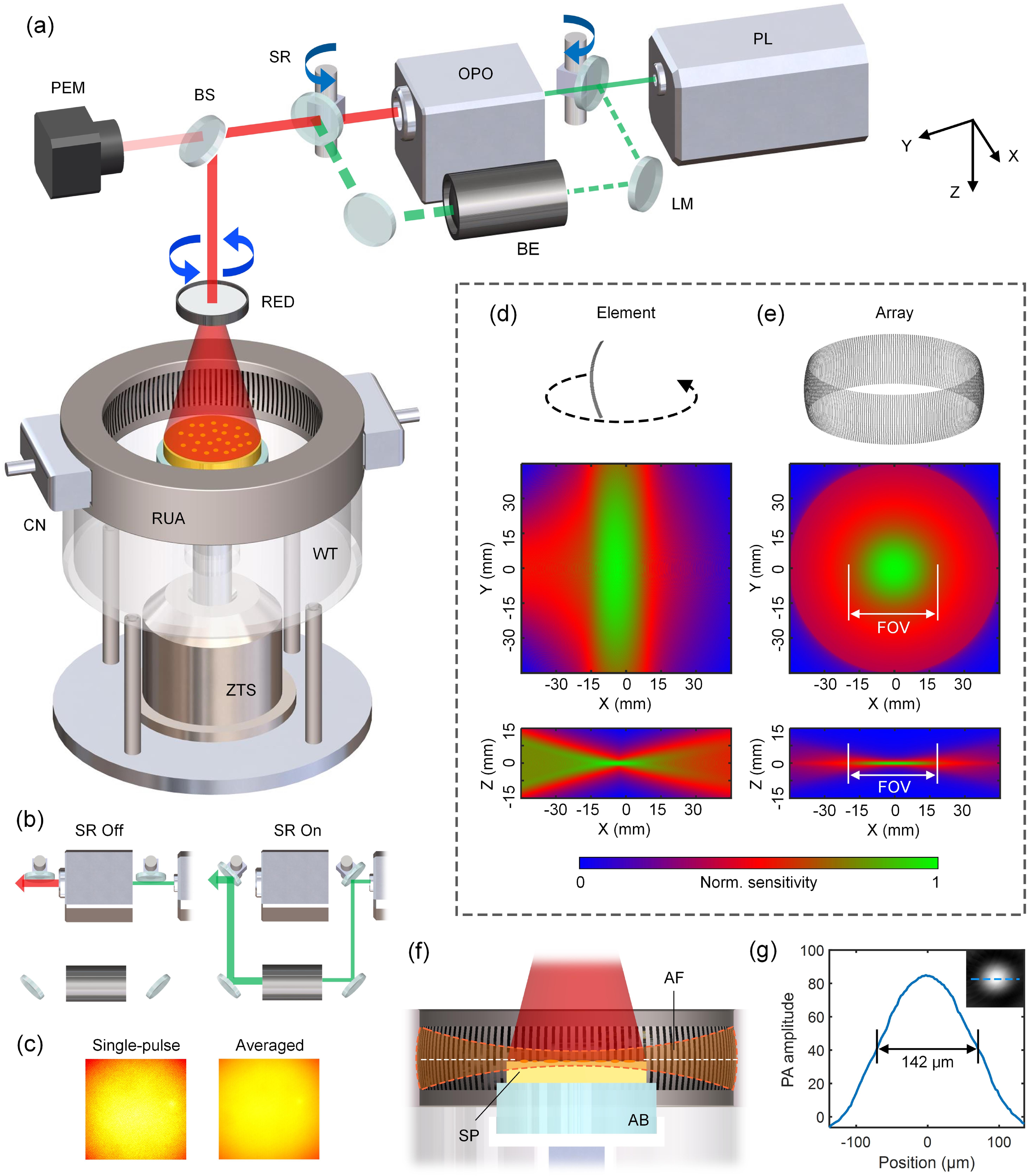
The layout of the SCAPAS setup is depicted in Fig. 1(a). The entire setup is composed of four main modules.

1. (1)Optical excitation module. A 532 nm laser (Nimma-900, 10-Hz pulse repetition rate, Beamtech Optronics Co., Ltd.) equipped with an optical parametric oscillator (OPO) (Continuum-OPO, Deyang Tech Co., Ltd) is used as the illumination source, providing ∼10ns pulse width at a fixed repetition rate of 10 Hz covering the near-infrared wavelength range of 650–900 nm. The OPO is pumped by the 532 nm laser with an energy conversion efficiency of approximately 20%. A pair of switchable reflectors driven by steering engines is adopted to enable dual-channel switching between visible and near-infrared illumination [Fig. 1(a)]. When the reflectors are switched to the “on” station, the 532 nm laser is directly through a series of mirrors to precisely align with the near-infrared output of the OPO. In this configuration, the OPO is inactive without the 532 nm pump. Conversely, when the reflectors are switched “off,” the 532 nm laser enters the OPO to produce near-infrared light [Fig. 1(b)]. A beam expander (Union Optic Tech Co., Ltd) is integrated into the bypass optical path to ensure the same beam diameter of the visible and near-infrared outputs. A 1:9 beam splitter redirects the coaxial laser beam to align parallel to the Z axis, while simultaneously channeling a portion of the laser energy to a pulse energy meter, enabling real-time monitoring of the energy fluctuation of the pulse train. The laser beam is then vertically incident on an engineered diffuser (EDC-10-G-1R, RPC Photonics Inc.), resulting in an output beam with a nearly flat-top intensity profile and a divergence half-angle of approximately 20°. By rotating the engineered diffuser at random speeds around its central axis with an external motor and averaging multiple pulses, speckles are further suppressed to achieve a more uniform light intensity distribution [Fig. 1(c)].
2. (2)Acoustic detection module. Distinguished from conventional screening platforms, SCAPAS features a 360° ring-shaped ultrasonic transducer array (Imasonic Inc.) that enables simultaneous acquisition of PA signals. The array has a radius of 50 mm and consists of 256 arc-shaped lead zirconate titanate (PZT) elements (50 mm radius, 26 mm height, and 0.5 mm width) with a central frequency of 5 MHz (−6dB two-way bandwidth >60%). The measured −6dB reception bandwidth ranges from 0.98 to 8.89 MHz [Fig. 8(c), Appendix A], which is sufficient to meet the imaging requirements for E. coli colonies. This design allows each element to focus along the elevational direction (Z axis) and achieve a substantial aperture angle in the X–Y plane [Fig. 1(d)], enabling the array to synthesize a disk-shaped acoustic field with a lateral diameter of ∼40mm and an elevational sectioning of ∼1.5mm [Fig. 1(e)]. This FOV is well-suited to the sample size used in the SCAPAS system (35 mm in diameter, determined by standard Petri dish specifications), ensuring uniform illumination across the sample [Fig. 1(f)].
3. (3)Data acquisition and control module. Two customized 128-channel preamplifiers (20 dB gain) are directly connected to the sides of the transducer array. The outputs from the preamplifiers are then fed into two 128-channel data acquisition (DAQ) boxes (Analogic Corp., SonixDAQ; 40 MHz sampling rate; 12-bit ADC; 36–51 dB programmable gain) for A/D conversion. The laser and the DAQ box are synchronized by a high-precision delay generator (Stanford Research Systems, DG645).
4. (4)Sample mounting module. A lab-made agarose base (4% mass fraction, 25 mm height) is used to support the samples, ensuring an acoustically transparent imaging cavity, and is connected to a Z-axis translation stage via a nylon holder for sample transport and positioning [Figs. 1(a) and 1(f)]. Phosphate-buffered saline (PBS) is used as the coupling medium to maintain the osmotic pressure balance within the cells of the E. coli sample.

The samples tested by SCAPAS consist of a culture substrate (∼4mm thickness) with a layer of E. coli colonies on its surface. Before the test, the Z-axis translation stage is moved to its uppermost position to facilitate sample placement. The stage is then lowered until the top surface of the sample aligns with the central plane of the transducer array [Fig. 1(f)]. During the dual-wavelength imaging process, the switchable reflectors initially remained in the off state and 20 frames of near-infrared (tunable output) PA data were acquired within 2 s. Subsequently, the reflectors are turned on and 532 nm PA data is collected in the same way. The laser pulse energy for each frame is correspondingly recorded by the energy meter. Averaging the raw data over 20 frames with pulse-energy-normalization boosted the SNR by 4.5 times while also achieving more uniform illumination [Fig. 1(c)], which facilitated the reconstruction of high-quality PA images. Overall, SCAPAS achieved a short screening time of 5 s per sample, translating to a throughput of 50 ms per colony (assuming an average of 100 colonies per sample). The lateral resolution (142 μm) of SCAPAS is calibrated using dyed polystyrene microspheres (5 μm diameter) positioned at the center of the FOV, which is sufficient for imaging E. coli colonies.

The reconstructed PA brightness (amplitude) of the ith colony, denoted by Img(i), is thus the product of SF and the real PA response of the T-GER, denoted by RPAT: Img(i)=SF(i)×RPAT(i).(2)

Due to the challenges in directly measuring SF (which depends on the colony index i), a traditional imaging-based readout method is unsuitable for accurate quantification of the PA response of T-GER, as illustrated in Fig. 2(c).

Here, we proposed a self-calibration method to alleviate the influence of SF. In SCAPAS, the reference genetically encoded reporter (R-GER) is introduced, which is designed to be co-expressed with T-GER in a 1:1 ratio, leading to a consistent spatial distribution of R-GER and T-GER within each E. coli colony [Fig. 2(d)]. The R-GER should satisfy two conditions: (1) the absorption peaks of R-GER and T-GER must be sufficiently separated to prevent absorption crosstalk at their respective peak wavelengths; (2) the R-GER molecule is required to exhibit a sufficiently strong PA response at its absorption peak. In fact, certain visible-light FPs can be selected as R-GER, as they exhibit negligible absorption in the near-infrared range and generate strong PA signals when excited with light around 500 nm. In dual-wavelength imaging of SCAPAS, employing the peak wavelengths of T-GER and R-GER for optical excitation (denoted by λT and λR) allows T-GER to contribute to the image (denoted by ImgT) at λT, while R-GER contributes to the image (denoted by ImgR) at λR. The spatial congruence between T-GER and R-GER ensures that they are both subject to identical systematic factors [Fig. 2(e)], allowing the images to be expressed as ImgT(i)=SF(i)×RPAT(i),(3)ImgR(i)=SF(i)×RPAR(i).(4)

For the sample of SCAPAS, all colonies express the same type of predetermined R-GER molecules, resulting in a constant RPAR across all samples: RPAR(i)=k.(5)

Thus, by combining Eqs. (3)–(5) to eliminate the influence of SF, RPAT can be linearly represented by the ratio of the dual-wavelength images, expressed as RPAT(i)=ImgT(i)kImgR(i)∝ImgT(i)ImgR(i).(6)

This self-calibration method employs an R-GER molecule coupled with each T-GER molecule to eliminate the influence of various systematic factors, thereby providing an effective means for evaluating RPAT. See Fig. 2(f) for an illustration.

The PA response of the expressed NIR-GERs under a certain wavelength can be modeled by assigning values to the voxels that constitute each colony (assuming a homogeneous spatial density of proteins). A numerical sample consists of multiple colonies, each of which can be assigned different morphological parameters and response intensity values, with all colonies sharing a common base plane. The digital imaging platform is constructed using the k-Wave toolbox of MATLAB 2021. The transducer configuration, frequency response, sampling rate, and other related parameters are consistent with those of the actual SCAPAS hardware. The ambient sound speed is uniformly set to 1500 m/s. The spatial grid size for the simulation is set to 50 μm, which reduces computational time while ensuring adequate spatial sampling to prevent aliasing. For the E. coli sample with a diameter of 35 mm, a single three-dimensional PA forward propagation simulation takes approximately 0.5 h (computer configuration: Intel Xeon Silver 4210R, 40 CPUs at 2.4 GHz, RAM 384 GB), generating a set of raw data with 256channels×1820time points.

In SCAPAS, the limited detection aperture and bandwidth lead to frequency loss in the reconstructed images, potentially causing the hollow artifacts shown in Fig. 3(c). To mitigate this, deconvolution is performed on the raw data to restore lost frequency components and improve image quality [24]. Here, we obtain the electronic impulse response (EIR) of the system using a rectangular thin-sheet absorber. A 10 mm long, 2 mm wide, and 200 μm thick absorber can be fabricated by preparing 50 mL 1% agarose solution mixed with 0.1 mL ink, followed by casting the mixture using a mold. The absorber is then embedded in transparent agarose and precisely aligned so that its largest surface coincides with the central plane of the transducer array, with the midpoint of one short edge positioned at the array’s geometric center [Fig. 8(a)]. This precise alignment is achieved by using a manual six-axis adjusting stage to control the position and orientation of the sheet absorber, while imaging it simultaneously. When the midpoint of sheet absorber’s short edge is aligned with the center of the FOV and the edges are most clearly imaged, it can be concluded that the sheet absorber coincides with the central plane (i.e., the focal plane). After alignment, the absorber is excited by uniform illumination at 532 nm, and the PA signals collected by the transducer elements directly facing the short edge are averaged over 1000 acquisitions to obtain an EIR waveform with high SNR. We simultaneously conducted simulations on the digital imaging platform, where absorbers are positioned and sized as described above with each voxel set to emit uniform PA signals. The simulated and measured results show high consistency in waveform width, indicating precise thickness control during absorber fabrication [Fig. 8(b)]. The slight differences in waveform oscillations and spectra are attributed to non-ideal uniformity in absorber concentration and optical excitation [Figs. 8(b) and 8(c)]. The thickness of the absorber ensures a large diffraction aperture, forming a nearly spherical wavefront matching the detector element’s surface. The material of the absorber prevents reflection artifacts caused by acoustic impedance mismatch. Compared to methods using point sources, the edge emits a unipolar wavefront rather than a bipolar one, allowing the acquired waveform to be directly used as the estimated EIR. The deconvolution is realized by applying a Wiener filter on the raw data applying the measured EIR. The FOV of SCAPAS can be further expanded by augmenting the number of transducer elements. Considering an FOV with a diameter denoted by Φ, the required element number (denoted by N) for the array (with the central ultrasound wavelength denoted by λc) can be calculated using the following formula [25]: N=2πΦλc.(8)

Based on the system parameters, it can be calculated that N≈800. Virtual channel data are generated by averaging adjacent channel data, augmenting the deconvolved 256-channel raw data to 512 channels. This method does not introduce additional information, but effectively reduces undersampling-induced streak artifacts, thus improving the accuracy of colony identification. Furthermore, since most colonies are regularly circular, it does not cause noticeable angular distortion. It should be clarified that array augmentation primarily reduces aliasing artifacts from image reconstruction rather than addressing physical spatial sampling limitations. These steps contribute to improving image quality, thereby enhancing the accuracy of imaging-based quantification methods.

With the deconvolved and augmented raw data, the PA images of SCAPAS are reconstructed by the universal back-projection (UBP) algorithms [26] implemented in MATLAB 2021. For simulation tests, the preset speed of sound (1500 m/s) can be directly used for image reconstruction. For practical tests, the speed of sound often fluctuates with slight changes in ambient temperature. Here, we draw on the concept of feature coupling algorithms [27], leveraging the symmetry of the ring array to iteratively search for the optimal speed of sound by maximizing the correlation between images reconstructed from two half-ring arrays as the optimization criterion. Due to the geometric regularity of the imaging sample and the relatively narrow range of sound speed iterations (1495–1505 m/s with a step size of 0.2 m/s), the risk of multiple local optima is mitigated. The pixel size for all reconstructions is set to 50μm×50μm, forming an image size of 700×700. To accelerate the image reconstruction, the UBP program is run on the GPU (CUDA version: 11.6, Quadro RTX 8000, NVIDIA). The reconstruction of a single image takes ∼0.1s, while a complete iteration of sound speed search and reconstruction takes ∼5s.

In experimental validation, two near-infrared FPs with weak fluorescence signals, iRFP713 and SNIFP, are employed as distinct T-GERs to assess the quantification capability of SCAPAS, with a red FP, mScarlet-H, serving as the R-GER. The samples were prepared following the steps outlined below.

1. (1)Construction of prokaryotic expression plasmids.The cDNAs of T-GERs (iRFP713/SNIFP) mutants and R-GER (mScarlet-H) are genetically fused by overlap extension PCR. The cDNA encoding a flexible peptide linker GGSGGS is introduced between iRFP713/SNIFP and mScarlet-H. The PCR fragments are cloned into the pRSET A plasmid by using the BamH I and EcoR I restriction sites. And then the PCR fragment of heme-oxygenase 1 (HO1) followed by ribosomal binding site (RBS) is amplified, digested, and introduced to the plasmid using EcoR I and Hind III restriction sites to produce the final expression plasmids pRSET- iRFP713-mScarlet-H-RBS-HO1 and pRSET-SNIFP-mScarlet-H-RBS-HO1. Q5 high-fidelity DNA polymerase (New England Biolabs) is used for routine PCR amplifications. Synthetic DNA primers for cloning are purchased from Tsingke Biotech (Beijing). All plasmids are sequenced before further analysis. The restriction enzymes are purchased from Thermo Fisher Scientific.
2. (2)DNA transformation and expression.Remove frozen BL21(DE3) pLysS competent cells from −70°C, and place them on ice for 5 min or until just thawed. Once the cells have thawed, add 3 ng of cDNAs of NIR-GER library or iRFP713 per 100 μL of competent cells. Record the injection time of each mutant plasmid. Quickly flick the tube several times, and then immediately place the tubes on ice for 30 min. Afterward, heat-shock the tubes in a water bath at 42°C for 90 s, followed by returning them to ice for 2 min. Next, plate the E. coli on SOB agar plates in chronological order to ensure consistent processing time for each mutant. Take care not to touch the edge of the plate. Allow the samples to grow overnight at 37°C. To complete the maturation process, leave the Petri dishes at 4°C for three days before imaging.

In this section, a numerical calibration sample is generated, and simulations are used to validate the effectiveness of image optimization as well as to illustrate the negative impact of systematic factors on the quantification of the PA response. In the calibration sample, each colony is modeled as a dome-shaped structure [28] defined by colony height H and base diameter D (refer to Section 2), with the radial position from the center of FOV denoted as R [Fig. 3(a)]. The PA response of FPs in all colonies is uniformly set to 1. In the upper half of the calibration sample, radially distributed colonies are arranged, all set to D=0.8mm. Ten angular positions correspond to ten different H values (50–500 μm with an interval of 50 μm), with seven identical colonies uniformly distributed radially along each angular position with different R values (4–12.4 mm with an interval of 1.4 mm). In the lower half, all colonies are set to H=200μm. Eight angular positions correspond to eight different D values, with three identical colonies uniformly distributed radially at each angular position with different R values (6–12.4 mm with an interval of 2.8 mm) [Figs. 3(b) and 3(i)]. The numerical calibration sample is imaged under the assumption of uniform illumination within the digital imaging platform, producing 256-channel raw data.

In the original image reconstructed from the 256-channel data, varying degrees of hollow artifacts are observed, along with increased artifacts in regions farther from the center of the FOV [Fig. 3(c)]. However, the fidelity of the images is significantly improved after applying deconvolution and array augmentation [Fig. 3(d)]. A section profile at the same position [labeled in Figs. 3(c) and 3(d)] allows for a direct comparison of the artifact suppression achieved through image optimization [Fig. 3(e)]. The standard deviations before and after optimization are 0.24 and 0.018, respectively, indicating that artifacts are suppressed by approximately 13 times. To further verify the suppression of hollow artifacts through image optimization, we selected colony images at three radial positions, labeled P1, P2, and P3, for comparison [corresponding to Figs. 3(f), 3(g), and 3(h), respectively]. By applying the two-dimensional Fourier transform to k-space, the loss of multiple frequency components is observed in the original k-space images, manifested as several depressions, which are the primary cause of the hollow artifacts. Additionally, colonies located closer to the transducer elements (i.e., farther from the center of FOV) exhibit slightly weaker low-frequency signal loss. This phenomenon may be related to the structure of the acoustic field of the array, where the thicker outer region has a greater weighting for capturing out-focus PA signals, thereby partially compensating for the loss of frequency component [29]. By applying the correct and high-SNR EIR waveform during deconvolution, the frequency depressions in the optimized k-space images are partially restored, with the spectra of the outer colonies in particular approaching an ideal Gaussian distribution [Fig. 3(h)]. The section profiles [labeled in Fig. 3(f)] more clearly demonstrate the improvements after optimization, closely resembling the profile of the preset ground truth after integration along the Z axis, which provides a foundation for imaging-based quantitative analysis.

The impact of systematic factors is analyzed through the images. The average pixel value within each preconfigured colony region can be used as the readout results. Although the PA response intensity of all colonies in the numerical sample is uniform (i.e., the voxels comprising the numerical sample are assigned the same value), significant differences are observed in the direct readout values due to the influence of systematic factors. The design of the calibration phantom allows us to study the relationship of H, D, R, and the readout values using the controlled variable method [Fig. 3(i)]. For colonies with the same H, the relationship between the readout value and D varies with R, which is a combination of the frequency response of the colony size within the transducer bandwidth and the spatial sensitivity of the acoustic field. For example, at R=12.4mm, a positive correlation is observed with the readout values exhibiting a disparity of up to 2.75 times due to the size change. In contrast, at R=6.8mm, the relationship transitions to a positive correlation followed by a negative one [Fig. 3(j)]. When D is fixed, the readout value exhibits a nonlinear variation with R [Fig. 3(k)], while it varies approximately linearly with H [Fig. 3(l)], indicating a positive correlation between the colony height and the readout values. Analysis of the calibration sample reveals that the direct readout results are significantly influenced by systematic factors, rendering them unsuitable for quantifying the PA response of FPs expressed by the E. coli colonies.

In this section, the quantitative capability of PA response in SCAPAS is validated by simulating the characteristics of real samples and the imaging process, followed by the application of self-calibration methods. For the numerical sample generation, the colonies are modeled as dome-shaped structures defined by base diameter D and height H [28]. We then construct numerical samples for quantitative simulations. The distributions of the colonies’ height and diameter are drawn from a distribution that represents real-world situations. We first select a colony with a representative diameter and observe its morphology under a bright-field microscope. By adjusting the focal depth of the microscope, the focus is on the substrate at z=0 and on the colony’s top at z=100μm [Fig. 9(a), Appendix A]. From this observation, we hypothesize that 100 μm would be a representative height of the colonies. We further observe the entire sample under a 690 nm fluorescence microscope and statistically analyze the distribution of the diameter of the colonies [Fig. 9(b)]. Based on these physical observations, the numerical sample is generated with D assigned within the range of 0.2–0.8 mm, with the similar distribution [Fig. 9(c)]. The base diameter and height are constrained by a relationship defined as H=βD, where β is a proportional coefficient randomly selected within the range of 0.17–0.4 [Fig. 4(a)], corresponding to the simulated height range from 34 to 320 μm [Fig. 4(a)], which encompasses the representative height of the actual colonies. The colonies’ positions are located within a circular area with a diameter of 35 mm, without overlaps. Then, the colonies in the numerical sample are divided into four regions according to the quadrants of the Cartesian coordinate system, with the PA response intensities of T-GER (refer to the NIR-GERs in real samples) set to 1, 1.3, 1.6, and 1.9 across Regions 1–4, respectively [Fig. 4(b)]. According to the design of the co-expressed sample, all colonies are assigned a uniform PA response of 1 for the same type of R-GER as a coupled reference. Thus, the numerical sample’s voxels are characterized by two distinct values, corresponding to T-GER and R-GER, respectively.

The dual-wavelength imaging of SCAPAS at λT and λR is simulated by separately acquiring reconstructed images of the numerical sample assigned with T-GER and R-GER voxel values [Figs. 4(c) and 4(d)]. Using the direct readout values of colonies from the λT image as the PA response intensity, the resulting distribution is chaotic, and it is not feasible to distinguish the PA response across different regions [Fig. 4(e)]. In the self-calibration method, the imaging results for each colony at λT and λR are individually extracted (denoted by ImgT and ImgR). To ensure computational stability, the non-negative least squares approach (NNLS) is employed instead of direct division to derive the PA response intensity (denoted by RPAT) of the ith colony, written as RPAT(i)=minRPAT(∥ImgR(i)−RPAT·ImgT(i)∥).(9)

The calculated results clearly reveal four distinct regions of T-GER PA response intensity [Fig. 4(f)], which correspond closely to the ground truth [Fig. 4(e)]. Evidently, the implementation of the self-calibration method has substantially improved the quantitative accuracy of SCAPAS.

For further validation, we establish four groups of T-GER PA response intensities and analyze the calculated results using box plots. Each group consists of four equidistant response values, corresponding to Regions 1 through 4 (Group 1: 1, 1.1, 1.2, 1.3; Group 2: 1, 1.3, 1.6, 1.9; Group 3: 1, 1.5, 2, 2.5; and Group 4: 1, 1.8, 2.6, 3.4). The ground truth (in red), the calculated results using self-calibration (in blue), and the direct readout results (in gray) are presented side by side in the box plot, with the latter two scaled relative to the mean value of their respective Region 1 results for a more intuitive comparison [Figs. 4(g)–4(j)]. The median-based analysis reveals that the maximum percentage deviation between the self-fabricated results and the ground truth is ∼3.8%. Within each region, the self-calibration results exhibit a maximum peak-to-peak fluctuation of 11.8% relative to the median value, with the largest observed standard deviation being 6.77%, which shows a fair consistency across different colonies. In Group 1, where the difference between the true values of PA response is preset to only 10%, the self-calibration method still demonstrated a remarkably high level of quantification accuracy [Fig. 4(g)]. In comparison, for Groups 1–3, the direct readout results exhibit negligible statistical significance, with poor consistency and a macroscopic trend that deviates substantially from the ground truth [Figs. 4(g)–4(i)]. For Group 4, the direct readout results appear to follow the same trend as the ground truth, allowing for a qualitative assessment of the relative response intensity. This can be attributed to the substantial disparity in the preset response values (80% for Group 4). However, in practical directed evolution processes, the incremental changes in protein characteristics between screening rounds are generally minimal, and the occurrence of such violent variations is infrequent. Consequently, the readout results reveal limited relevance in practical experimental applications.

By adding Gaussian white noise into the dual-wavelength raw data, we evaluated the impact of SNR on the quantitative performance of SCAPAS. We compared the zoomed-in regions [labeled in Fig. 4(c)] of reconstructed images corresponding to raw data with SNR of 2, 8, 15, and 30. For low-SNR images, noise overlays the colonies, altering the original pixel values, which may diminish the quantification accuracy to some extent [Fig. 4(k)]. By comparing the performance of the self-calibration method across different SNRs (based on Group 2), it is observed that when the SNR drops to 2, the maximum percentage deviation of the median from the ground truth increases to 9.23%, and the percentage fluctuation relative to the median rises to 36.5%, as evidenced by the broadening in the box plot [Fig. 4(l)]. This indicates that even poor image quality can still support acceptable quantification results. Therefore, during the SCAPAS imaging process, averaging methods are employed to ensure sufficient SNR (refer to Section 2). We further compare the impact of signal deconvolution on the quantification results (Fig. 10, Appendix A). It can be observed that after deconvolution, the quantification accuracy does not change significantly, but the precision improves (i.e., the narrowing of the box) [Fig. 10(c)]. This may be attributed to the hollow structure of the colonies in the original images, which results in the inner regions of the colonies being primarily influenced by noise during the self-calibration calculation, thereby significantly reducing precision [Figs. 10(a) and 10(b)].

The morphology of the colonies is influenced by factors such as the composition and concentration of the culture medium, temperature, as well as the spatial density of the colonies (i.e., the amount of free space occupied by each colony) [28]. Furthermore, the colony morphology evolves over time [30]. As a result, in high-throughput directed evolution screening, strict control of experimental conditions is essential to minimize sample variations. Specifically, the samples must be cultured in identical media, under the same conditions, and for the same duration, to ensure highly homogeneous colony morphology, as described in the previous section. We realize that colony morphology could potentially influence the detected PA signal strength, which we have modeled using the Morph term in Eq. (1). However, in SCAPAS, the influence of the Morph term is eliminated during the quantification process. While the colonies are modeled as dome shapes, we have validated that the SCAPAS procedure (through which the influence of Morph is eliminated) is independent of the exact shape of the colonies. This is because the Morph term is a wavelength-independent geometric factor, which can be canceled when Eq. (6) is applied. To clarify, we simulate two groups of samples with identical spatial distributions and parameters, with the only difference being the colony shape. One group consists of dome-shaped colonies [Fig. 11(a), Appendix A], while the other exhibits a flat-topped geometry [Fig. 11(b)]. After applying the self-calibration method to both groups, no significant difference is observed between the two groups [Fig. 11(c)].

In the experimental validation, two FPs with weak fluorescence signals, iRFP713 and SNIFP, are selected as T-GERs to prepare two types of E. coli colony samples, which are used to assess the quantification capabilities of SCAPAS. A red FP, mScarlet-H, is co-expressed with T-GER as R-GER (refer to Section 2). The absorption spectra of iRFP713, SNIFP, and mScarlet-H indicate that imaging at dual wavelengths of 532 and 690 nm ensures robust PA signals for these FPs, while effectively minimizing signal crosstalk [Fig. 5(a)]. To further evaluate potential crosstalk, preliminary experimental samples are prepared with four distinct regions. One region served as a control with no expression, while the remaining three regions expressed each of the applied proteins individually. Imaging is then conducted using SCAPAS at the selected wavelengths, and no significant signal crosstalk is observed between iRFP713/SNIFP and mScarlet-H [Fig. 5(b)]. The imaging results also indicate that E. coli itself produces negligible signals at both wavelengths, ensuring that the PA signals generated from the samples are solely attributable to the light absorption of the expressed proteins [Fig. 5(b)].

To establish a ground truth for PA response intensity, iRFP713 and SNIFP are purified from E. coli samples and prepared into solutions with identical molar concentrations. For each T-GER, the solutions are injected into polytetrafluoroethylene (PTFE) microtubes with an inner diameter of 200 μm, and continuous imaging is performed for 30 s, yielding 300 reconstructed frames [Fig. 5(d)]. By calculating the averaged pixel value within the cross-sectional area of the microtubes, a time-dependent curve of the purified protein’s PA signal can be generated [Fig. 5(c)]. It can be observed that under continuous pulsed laser exposure, the PA signals of T-GERs remain relatively stable during the first 50 frames (corresponding to the first 5 s), after which varying degrees of photobleaching occur, manifested as a gradual decrease in PA signal. During the testing of E. coli samples using SCAPAS, the imaging duration is limited to 2 s, remaining within the non-photobleaching range. This ensures the stability of T-GER signal values over time, thus maintaining the accuracy and reliability of the quantification results [Fig. 5(c)]. By calculating the averaged signal of the first 20 time points on the curve, the ground truth of PA response ratio of the two T-GERs can be obtained (SNIFP 0.79, normalized to iRFP713 PA response) and used as a comparison for the quantification results of the E. coli colony samples [Fig. 5(e)].

In practical tests, E. coli colony samples expressing iRFP713 and SNIFP with mScarlet-H as the co-expressed reference are prepared. Five replicates of each sample are produced to verify the reproducibility of the experimental results, with the total number of colonies per sample controlled at approximately 100–200. In SCAPAS, data acquisition for an individual sample is completed within 5 s, producing high-quality dual-wavelength PA images with an average SNR of approximately 15 (refer to Section 2). To localize the colony regions, the Hough transform is employed to identify circular regions in the images. Due to the existence of spatial response, E. coli colonies located near the edges of the FOV exhibit shape distortions, making them difficult to identify, which can hardly affect the overall statistical analysis. For each identified position, local dual-wavelength images are extracted, and the correlation coefficient is calculated. If the value exceeds 0.9, the region is considered a valid colony position; otherwise, it is classified as a false-positive. This process is repeated to filter and finalize the positions of valid colony regions [Fig. 6(a)]. With the locations determined, the direct-readout PA responses are obtained from the 690 nm images. The PA responses using the self-calibration method are also calculated from the dual-wavelength images. These values are then assigned to the corresponding colony regions to create a PA response intensity map [Fig. 6(a)]. For clearer visual comparison, the intensity maps of each method are normalized to the mean of the corresponding iRFP713 samples, allowing the use of a shared colorbar [Figs. 6(a) and 6(b)].

By comparing the intensity maps generated from all tested samples, it is evident that the self-calibration results readily differentiate between the two types of T-GERs. Specifically, the intensity map for iRFP713 is clearly brighter than that of SNIFP. In contrast, the direct readout results do not allow for a visual distinction between the two types of T-GERs, as no observable differences are present [Fig. 6(b)]. By plotting all results using box plots, it becomes clearer that the self-calibration method can distinctly separate the two groups of E. coli samples expressing different T-GERs [Fig. 6(c)], whereas the direct-readout method struggles to achieve this [Fig. 6(d)]. It is important to note that in SCAPAS, different quantification methods can produce varying results for the same type of T-GER. As such, the absolute PA response intensities do not carry direct physical significance and should be expressed as ratios relative to a reference T-GER (e.g., iRFP713 in this case) for meaningful comparison. A T-test matrix is also constructed by calculating the p-values between any two sets of results. If the p-value is less than 0.05, the corresponding position is marked as 1 (indicating statistically significant differences); otherwise, it is marked as 0. For self-calibration results, samples expressing the same type of T-GER are almost tested as from the same population (marginal statistical differences), while samples of different types of T-GERs are tested as originating from different populations, indicating significant differences that align with the natural facts [Fig. 6(e)]. However, in the readout results, there is a weak correlation among samples of the same T-GER, while some correlation is observed among samples of different T-GERs, which contradicts the expected outcome [Fig. 6(f)].

We further conduct statistical analysis on the results of the self-calibration method and evaluate the quantification capability of SCAPAS for PA responses. Considering SCAPAS as an estimator of the PA response intensity for NIR-GERs expressed by each colony, its quantification capability can be assessed in two dimensions. The first is precision, which reflects the variability of the estimator across different samples from the same population and is typically measured by the standard deviation. The second is accuracy, which reflects the deviation of the estimated values from the true value and is quantified by the bias. We first calculate the standard deviation for the quantification results of each E. coli sample [Fig. 7(a)]. Although the standard deviation is determined by the systematic characteristics of the estimator, increasing the number of statistical samples can help approximate the true standard deviation. The standard deviation is also independent of the selected population. As illustrated in Fig. 7(a), there is no statistically significant difference in the standard deviation between the two groups of samples expressing different T-GERs. By aggregating the five samples expressing the same T-GER into a larger population, two standard deviations can be derived (shown in arrows, 0.2619 and 0.2185), and the larger one is selected as a conservative upper-bound estimate of standard deviation (0.2629). We then calculate the mean value for the quantification results of each E. coli sample [Fig. 7(b)], and, similarly, the mean values for both populations are provided (shown in arrows, 4.065 and 3.228). Given that the PA response intensities in SCAPAS do not possess direct physical significance, the aforementioned statistical results should be transformed into metrics that facilitate a more rigorous and intuitive evaluation of the system’s quantification performance. Using iRFP713 as a reference, and considering that the PA response of the desired NIR-GERs exceeds that of iRFP713, we can obtain the upper-bound of the relative standard deviation (6.47%) by dividing the standard deviation (0.2629) by the mean response of the iRFP713 samples (4.065), serving as a metric to characterize the quantification precision. To assess accuracy, we calculate the PA response ratio by comparing the mean values of each SNIFP group with those of the iRFP713 group. The percentage deviation from the ground truth (0.79) is then determined, forming a bias matrix [Fig. 7(b)]. The results show that the bias does not exceed 2.8%, which is relatively a conservative estimate. In summary, through empirical testing of E. coli samples and comparison with established ground truth, the superior performance of SCAPAS in quantifying PA response intensity has been validated from multiple perspectives.

In this study, we present SCAPAS, a platform capable of rapidly and accurately quantifying the PA response intensity of NIR-GERs expressed by E. coli samples. To the best of our knowledge, it is the only method currently available in the field that can achieve this functionality. SCAPAS quantifies the PA response level of individual GER molecules, which represents the most fundamental evaluation criterion for photoacoustically compatible GERs. As an imaging-based quantification method, SCAPAS incorporates unique designs in its system architecture, image reconstruction, and data analysis. SCAPAS is capable of completing data acquisition for an E. coli sample within 5 s (equivalent to 50 ms per colony), reconstructing high-quality dual-wavelength images with an FOV exceeding 35 mm in diameter and a spatial resolution of 200 μm. It can be concluded that SCAPAS achieves a considerable quantification accuracy of approximately 2.8% when screening novel NIR-GERs with PA responses stronger than iRFP713, along with a quantification precision of about 6.47%. Here, the quantification performance is assessed through statistical analysis of a large sample set from a defined population, with the resulting metrics providing predictive insights into the SCAPAS’s quantification capability for individual NIR-GERs expressed by single colonies. This closely reflects practical screening applications where each colony expresses a distinct type of NIR-GER. The system’s accuracy and precision are adequate to meet the requirements of most screening scenarios, as individuals with minimal improvement compared to iRFP713 will not proceed to the next round of iterative screening. These characteristics position SCAPAS as a promising pathway for facilitating the directed evolution of NIR-GERs with strong PA responses, specifically tailored for PA imaging.

However, some errors affecting accuracy persisted. For all results, the box plots exhibit broadening rather than reaching the ideal single value, which reduces the quantification accuracy to some extent. A potential systematic error source may stem from the inconsistency in the dual-wavelength illumination, which is caused by the refractive index differences of the engineered diffuser and the chamber fluid at different wavelengths. As shown in Fig. 12 (Appendix A), the differences in dual-wavelength light intensity distribution are indiscernible in the grayscale colormap but become visible when mapped with relative difference. This inconsistency may lead to errors in the quantification results, as the light intensity term cannot be eliminated in the self-calibration method. To validate this hypothesis, we conduct simulations using the controlled variable method to investigate the effects of inconsistencies in the dual-wavelength intensity distribution. The simulated illumination distribution is set based roughly on the real illumination patterns and the magnitude of relative differences [Fig. 13(a), Appendix A]. Results from the self-calibration method indicate that, compared to the case with strictly consistent illumination, the slight differences in light intensity distribution introduced some quantification errors, as evidenced by the broadening of the box plots [Fig. 13(b)]. A potential solution involves using precise beam shapers and expanders instead of diffusers to homogenize light intensity while achieving near-collimated illumination, thereby reducing the light distribution discrepancies caused by refractive index differences. This may enhance the consistency of quantification results for the same type of NIR-GER (i.e., the narrowing of the box plots). Additionally, numerical simulations show that image quality also impacts quantification results. While self-calibration methods tolerate variations in SNR, higher SNR undeniably results in more accurate quantification. Therefore, we intentionally sacrificed imaging speed during the process to increase the SNR by approximately 4.5-fold within the non-bleaching range. In experimental testing, we found that E. coli colonies located at the edge of FOV could not be identified via Hough transform due to distortions caused by the spatial impulse response function, leading to a reduction in the number of colonies included in the statistical analysis for a given sample. More advanced reconstruction methods, such as model-based iterative reconstruction [31,32], may potentially incorporate this factor into the forward model to mitigate distortion, though this comes at the cost of dramatically increased computational complexity.

SCAPAS is applicable to situations with more complex absorption spectra where spectral overlap exists between the absorption spectra of T-GER and R-GER. However, it is essential to ensure that no spectral overlap occurs at the two selected imaging wavelength points. This is a necessary condition for SCAPAS to achieve quantitative screening. As shown in Fig. 5(a), although there is some overlap in the absorption spectra of the T-GER (iPFP713 or SNIFP) and R-GER (mScarlet-H) used in this study, they are completely independent at the two imaging wavelengths of 532 and 690 nm. In fact, this condition is easily met because the center wavelengths of T-GER and R-GER are far apart, and the absorption spectra of GERs are generally narrow-band, making it easy to select two imaging wavelengths that are free from overlapping. In this study, R-GER is chosen as a reporter with an absorption peak at a shorter wavelength (e.g., mScarlet-H), while T-GER has an absorption peak at 690 nm, which is still relatively short for the PA imaging window (700–1100 nm). Therefore, the ability to independently excite the target and reference GER is generally achievable. However, in the rare instances where there is significant spectral overlap between T-GER and R-GER, independently exciting R-GER may prove challenging. This difficulty arises because independently exciting T-GER is typically easier, given that the absorption spectra of chromoproteins are much sharper on the red edge. In such cases, a T-GER photobleaching strategy can be employed: by independently and continuously exciting T-GERs until they are photobleached, one can then proceed to independently excite and image R-GER. This method is analogous to the acceptor photobleaching technique commonly used in fluorescence resonance energy transfer (FRET) imaging [33].

In SCAPAS, the selection criteria for R-GER are as follows: its absorption spectrum must be distinguishable from that of T-GER, with a sufficiently strong PA response and good stability. We chose mScarlet-H as the reference protein for the following reasons: (1) it has a short central absorption wavelength, with a spectrum clearly distinguishable from that of T-GER [Fig. 5(a)], making 532 and 690 nm—two common wavelengths for PA imaging—suitable for independently exciting T- and R-GERs; (2) mScarlet-H’s PA response at 532 nm is sufficiently strong, with a high imaging SNR; and (3) mScarlet-H is one of the most stable red fluorescent proteins available [34]. In the self-calibration method, since the PA readout from R-GER appears in the denominator, a high SNR is required. Therefore, an ideal candidate for R-GER should exhibit a strong PA response, which enhances the quantification accuracy of T-GER, as verified by our numerical simulations [Figs. 4(k) and 4(l)]. The stability of R-GER also impacts quantification accuracy. For example, differences in the photobleaching rates of R-GER and T-GER can complicate the self-calibration process, thereby reducing quantification accuracy. Fortunately, the 5-s imaging duration of SCAPAS is short enough to minimize inaccuracies caused by such sample instabilities.

It is crucial to emphasize that SCAPAS represents a comprehensive design that relies on the precise coordination of sample preparation, the imaging system, and the reconstruction algorithm. Unlike traditional samples, in SCAPAS, the T-GERs are co-expressed with R-GER, providing a fundamental basis for accurate quantification of the PA response. In contrast to conventional screening systems that utilize single-point excitation with scanning detection for imaging, SCAPAS leverages a ring ultrasonic transducer array coupled with wide-field illumination, enabling parallel detection. Its advantages extend beyond the rapid imaging of individual samples. The short imaging time reduces the risk of photobleaching and colony dissolution, both critical factors that impede quantitative screening. In addition, the frequency response of the transducers is tailored to match the characteristics of the imaging object. The diameter of E. coli colonies ranges from approximately 0.2 to 0.8 mm. Using the inverse relationship with the speed of sound in water (1500 m/s), the ideal frequency range can be estimated to cover 1.875–7.5 MHz. It needs to be clarified that the transducers in SCAPAS have a center frequency of 5 MHz with a two-way bandwidth of no less than 60% (as tested in the transmit–receive mode by the manufacturer). Based on the relationship that the one-way bandwidth (i.e., the photoacoustic mode with signal reception only) is 2 times the two-way bandwidth, the applied bandwidth can be calculated to be no less than 85%, corresponding to an available frequency range of at least 2.05–7.95 MHz. This design essentially corresponds to the ideal frequency range required for imaging E. coli colonies. Furthermore, the measured one-way frequency range of 0.98–8.89 MHz is larger than the theoretical range, clearly meeting the imaging requirements. To facilitate dual-wavelength imaging of the co-expressed molecules, SCAPAS incorporates a rapid wavelength-switching capability. With these prerequisites in place, self-calibration methods can be effectively employed, yielding accurate quantification results. By utilizing the imaging results of the reference molecules (i.e., the imaging contrast derived from the reference molecules), it is possible to precisely cancel the influences of various unideal imaging factors, and the desired NIR-GERs are screened from numerous T-GERs. Similar concepts have also been employed in methods such as Western blotting [35,36]. Apart from unideal systematic factors, the quantification ability of PA modality also remains controversial [37,38], which further underscores the necessity of employing self-calibration methods.

An additional critical consideration is the operational workflow of the SCAPAS for practical NIR-GER screening and its extended design. In actual high-throughput screening, the imaging process involves five steps for each sample plate: (1) sample placement, (2) dual-color PA imaging, (3) data processing, (4) colony picking, and (5) sample removal. The imaging and data processing times are as follows: imaging takes about 5 s, image reconstruction takes about 5 s, and colony recognition along with signal self-calibration takes about 2 s. The remaining parts of the screening process primarily involve sample delivery and retrieval. Currently, we manually load and retrieve the samples, which takes approximately 20 s. However, this process can be accelerated. For example, several fluorescent-based screening platforms utilize delta robot arms with specialized picking heads to efficiently and precisely select high-signal colonies [39]. With automated sample handling, the entire SCAPAS screening process for a single sample plate is expected to take no more than 30 s. For the newly screened NIR-GERs, a series of PA imaging validations is also necessary to evaluate their performance in in-vivo applications. In addition, based on the same system and methodology, the screening focus of SCAPAS can be further expanded from FPs to chromophore proteins [40,41], providing more chances for obtaining desired proteins. SCAPAS has universal applicability for genetically encoded reporters (GERs). These endogenous reporters can be expressed within cells through gene expression, using E. coli as a universal carrier and thus are compatible with the SCAPAS screening and the quantification process with self-calibration.

In summary, we present SCAPAS, a novel concept capable of rapidly and accurately quantifying the PA response of NIR-GERs expressed by E. coli samples. Through the synergistic design of the system and algorithm, the newly introduced system is ideally suited for the development of novel NIR-GERs with strong PA response, enabling rapid quantification of NIR-GERs in each screening round, thereby supporting the accurate execution of directed evolution. We believe that SCAPAS has the potential to profoundly impact the advancement of PA probes and molecular imaging, ultimately supporting the visualization of deeper and more diverse in-vivo functions with optical specificity.