Fig. 1. Experimental setup. A fiber coupled light emitting diode (LED) at telecom wavelength (1) inputs a motorized spectral filter (2), a 50 dB attenuator (3) and is split by a fiber beam splitter (4) to generate strong S beam simulating the star and weak P beam simulating exoplanet. The S beam is carved from LED using a fiber coupled filter (5) and free space launched with collimator (S); the P beam is free space launched with collimator (P) and carved using the free space spectral filter (6). Both beams cross two-lens (L) systems to match the beam waist with demultiplexer waist (300 μm) and are coupled with it by means of two steering mirrors each. The P beam crosses a film polarizer mounted on a motorized rotation stage (7) to control the beam intensity. The second mirror of the P beam is placed on a micrometer translation stage (8) to shift the beam position and so change the S and P separation in a controlled way. S and P beams are recombined on a beam splitter (9) and, after crossing a fixed film polarizer (7’), are coupled with demultiplexer. This polarizer is used to keep fix the photons polarization during the experiment to prevent polarization dependence of detection efficiency. The demultiplexer (10), PROTEUS-C from Cailabs, allows to perform intensity measurements on six HG modes; however, just the HG01, HG10, and HG00 modes are detected through three superconductive nanowires single-photon detectors (11) whose electrical output signal is detected and counted by a time tagger (12). Three polarization-rotation paddles for detectors efficiency maximization are inserted between demultiplexer fiber outputs and nanowires fiber inputs and optimized at the beginning of the experiment.

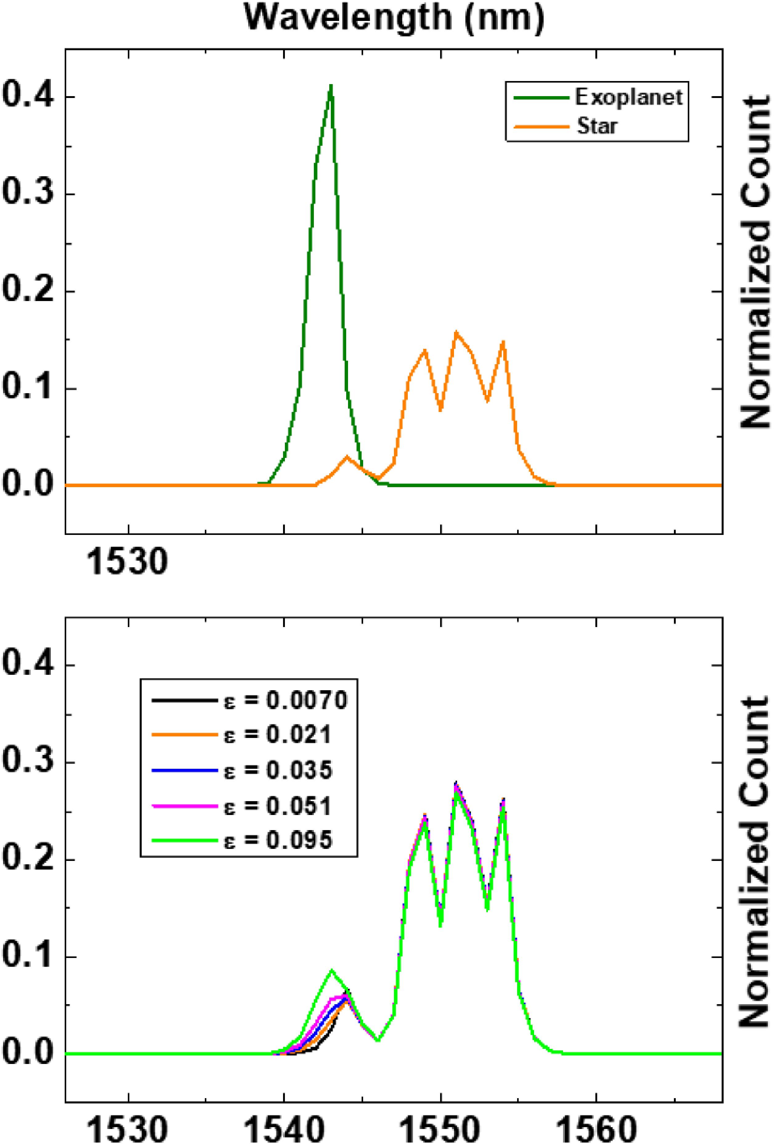
Fig. 2. Point-like sources spectra. The figure (upper panel) shows the spectra, obtained by normalizing single-photon counts, of two pointlike sources simulating the star (orange line) and exoplanet (green line). The scan over the wavelength is performed using motorized fiber-coupled spectral filter with 1 nm as minimum settable step size. The lower panel represents the real emitted normalized star–planet spectra at different values of intensity ratio ϵ.

Fig. 3. HG demultiplexed spectra at fixed ϵ. The figure shows the spectra of zeroth order (upper) and first order (lower) HG modes obtained by normalizing the counts C0N and C1N, respectively, as described in the text, at five values of separation da and fixed ϵ=0.021. The C1N spectra show a strong dependency on da proving the effectiveness of HG SPADE in spectroscopy of sources emitting spatial (without circular symmetry) dependent spectra. Inset shows a magnification of the wavelength region due to simulated exoplanet emission where the dependency is even more clear.

Fig. 4. HG demultiplexed spectra at fixed da. The figure shows the spectra of zeroth order (upper) and first orders (lower) HG modes obtained by normalizing the counts C0N and C1N, respectively, as described in the text, at five values of sources intensity ratio ϵ and fixed separation da. The C1N spectra show strong dependency on ϵ proving the effectiveness of HG SPADE in spectroscopy of sources emitting spatial (without circular symmetry) dependent spectra. Inset shows a magnification of the wavelength region due to simulated exoplanet emission where the dependency is even more clear.

Fig. 5. Scalar product quantifier. The data points show the experimentally estimated scalar product defined in Eq. (33), plotted as a function of da at fixed ϵ; SP(da,ϵ=0.021). The error bars are estimated by repeated measurements and take only into account statistical errors (about 0.01). At da=0 the scalar product is slightly lower than unity (about 0.98) because of systematic uncertainty that is not considered in error bars. By considering statistic (about 0.01) and systematic uncertainties [1−SP(da=0)], we have an overall uncertainty of about 0.03; as such, we can affirm that, when HG scalar product is below 0.97 (for da larger than 0.2), the SPADE technique can distinctly discriminate between star and exoplanet. The solid line shows the analogous quantity computed in the case of direct imaging. In the case of DD, a comparable discrimination capability is achieved when da is larger than 2.

Fig. 6. Scalar product quantifier. The data points show the experimentally estimated scalar product in Eq. (33), plotted as a function of ϵ at fixed da; SP(da=0.33, ϵ). The error bars show our estimate of the statistical errors. The error bars are estimated by repeated measurements and take only into account statistical errors. At ϵ=0, the scalar product is lower than unity (about 0.92) because of systematic uncertainty that is not considered in error bars. By considering statistic (about 0.01) and systematic [1−SP(ϵ=0)] uncertainties, we have an overall uncertainty of about 0.09. We argue that, when the HG scalar product is below 0.91 (when ϵ is larger than 0.008), the SPADE technique can distinctly discriminate between star and exoplanet. The solid line shows the analogous quantity for DD, which is close to 1 across all the range up to ϵ=0.1.