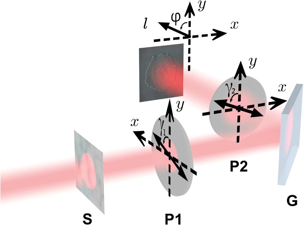
Fig. 1. Schematic of the phase-mining method based on polarization analysis of light reflection on a dielectric interface, e.g., an air–glass interface. A phase object S is uniformly illuminated and then the light is polarized by a polarizer P1 and reflected on the surface of a glass slab G. By analyzing the polarization of the reflected light with a polarizer P2, the differential contrast image of S appears at the imaging plane of the system and can exhibit a shadow-cast effect. The polarizers P1 and P2 are orientated at the angles ${\gamma }_1$ and ${\gamma }_2$. The direction of the spatial differentiation is along $l$ and indicated with an angle $\phi$.

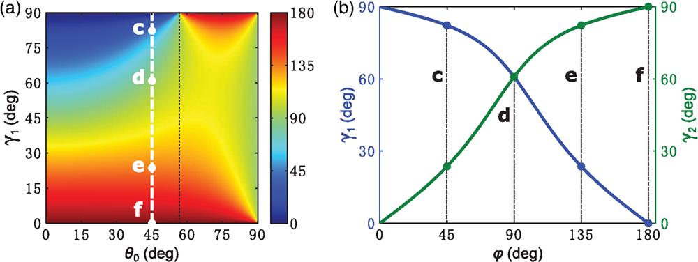
Fig. 2. Adjustability demonstration of the direction angle $\phi$. As an example, here the source is a green laser with wavelength $\lambda =532\mathrm{nm}$ in vacuum and a BK7 glass slab with refractive index 1.5195 is used for reflection. (a) Adjustable range of direction angle $\phi$ under a certain incident angle ${\theta }_0$ with different pairs of ${\gamma }_1$ and ${\gamma }_2$ satisfying the cross-polarization condition. The white and black dashed lines correspond to ${\theta }_0=45\mathrm{deg}$ and the Brewster angle, respectively. The points c to f on the white dashed line correspond to $\phi =45\mathrm{deg}$, 90 deg, 135 deg, and 180 deg, respectively. On the white dashed line in (a), ${\theta }_0=45\mathrm{deg}$. (b) Specific values of ${\gamma }_1$ and ${\gamma }_2$ for a certain direction angle $\phi$. The points c to f are the same as those in (a), corresponding to $\phi =45\mathrm{deg}$, 90 deg, 135 deg, and 180 deg, respectively.

Fig. 3. Measurement of spatial differentiation results and corresponding spatial spectral transfer functions along different directions. (a)–(d) Measured spatial differentiation results of the phase distribution [the inset in (a)] along different directions with $\phi =45\mathrm{deg}$, 90 deg, 135 deg, and 180 deg, corresponding to points c to f in Fig. 2(a), respectively. The inset in (a) is a disc test pattern with different phases for the gray and the white areas. (e)–(h) Experimental results of spatial spectral transfer functions, corresponding to (a)–(d). (i)–(l) Corresponding theoretical results calculated based on Eq. (3).

Fig. 4. Experimental demonstration of bias introduction and shadow-cast effect in differential contrast imaging of phase objects. (a) Theoretically calculated bias values under different ${\gamma }_1$ and ${\gamma }_2$. The black dashed curve corresponds to the cross-polarization condition, where the bias value $b=0$. (b) Phase distribution on the SLM, converted from an epithelial cell’s image. (c) Schematic of a virtual light source obliquely illuminating an object (green). The shadow-cast effects with virtual illumination from the points d to g schematically correspond to those in the biased images (d)–(g). (d)–(g) Measured biased differential contrast images with positive bias values corresponding to the triangle points d to g in (a), with bias values $b=0.0163$, 0.0151, 0.0100, and 0.0054, respectively. The white arrows indicate the orientations of the shadow cast in measured images. The white bars correspond to the length of $100\mu \mathrm{m}$.

Fig. 5. Directional derivatives of phase distribution in Fig. 4(b) and the corresponding recovered phase. Experimental results of (a) vertical and (b) horizontal partial derivatives of phase distribution in Fig. 4(b). Ideal (c) vertical and (d) horizontal partial derivatives. (e) Recovered phase distribution from (a) and (b) using the 2-D Fourier algorithm. (f) Original phase distribution on the SLM [the same as Fig. 4(b)].