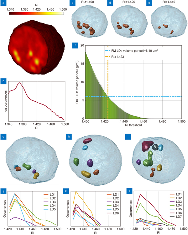
Fig. 1. Segmentation of the LDs within the 3D RI tomograms of A2780 live cells. (a) Central slice of the 3D RI tomogram of an A2780 live cell, in which LDs take the highest RI values. (b) Histogram in logarithmic scale of the 3D RI distribution of the cell in (a). (c–e) Isolevels representation of the tomogram in (a), in which LDs (orange) have been segmented by using the RI thresholds reported above. (f) Average volume per cell of the LDs segmented in 54 TPM tomograms of A2780 live cells by using different RI thresholds. The selected LDs-threshold (yellow line) allows computing the same average volume measured in 2D FM images (blue line). (g–i) Isolevels representation of separated LDs or LDs clusters segmented in 3 A2780 tomograms by using the LDs-threshold selected in (f), and (j–l) corresponding RI histograms. (a–e,g–j) are the same cell.

Fig. 2. LDs features extracted from 54 A2780 3D RI tomograms. (a–e) Histograms of respectively the mean value, standard deviation, entropy, kurtosis, and skewness of the 3D RI distributions of each LD. (f–h) Histograms of respectively the equivalent radius, the dry mass, and the sphericity of each LD. (i) Histogram of the distance between each LD centroid and the corresponding cell centroid, normalized to the cell equivalent radius. (j) Histogram of the distance between each LD centroid and the centroid of all the LDs inside the same corresponding cell, normalized to the cell equivalent diameter. (k) Mean RIs (orange dots) of concentric inner zones (orange regions) selected inside the same LD, with overlapped in blue the parabolic fitting. (l) Bivariate histogram of the first and second order coefficients of the parabolic fitting in (k) measured in all the LDs (black dots).

Fig. 3. Segmentation of the LDs within the 3D RI tomograms of THP-1 live cells. (a) Average volume per cell of the LDs segmented in 34 TPM tomograms of THP-1 live cells by using different RI thresholds. The selected LDs-threshold (yellow line) allows computing the same average volume measured in 2D FM images (blue line). (b, c) QPMs of two THP-1 cells, one without LDs (b) and the other one with LDs (c) (dark red spots). Scale bar is 5 μm. (d, e) Central slices of the 3D RI tomograms of the cells in (b,c), respectively, in which LDs take the highest RI values (Supplementary Movie 1). (f) Histogram in logarithmic scale of the 3D RI distribution of the cells in (d) (yellow) and (e) (red). (g) Isolevels representation of the tomogram in (e), in which LDs (orange) have been segmented by using the LDs-threshold selected in (a) (Supplementary Movie 2).

Fig. 4. LDs features extracted from 34 THP-1 3D RI tomograms.(a–e) Histograms of respectively the mean value, standard deviation, entropy, kurtosis, and skewness of the 3D RI distributions of each LD. (f–h) Histograms of respectively the equivalent radius, the dry mass, and the sphericity of each LD. (i) Histogram of the distance between each LD centroid and the corresponding cell centroid, normalized to the cell equivalent radius. (j) Histogram of the distance between each LD centroid and the centroid of all the LDs inside the same corresponding cell, normalized to the cell equivalent diameter. (k) Mean RIs (orange dots) of concentric inner zones (orange regions) selected inside the same LD, with overlapped in blue the parabolic fitting. (l) Bivariate histogram of the first and second order coefficients of the parabolic fitting in (k) measured in all the LDs (black dots).

Fig. 5. Conventional 2D imaging of A2780 (a–f) and THP-1 (g–l) live cells. (a, g) TEM images of LDs. Scale bar is 0.5 μm. (b, h) Representative FM images of nuclei (blue) and LDs (green). Scale bar is 10 μm. (c, i) FM images of nuclei stained with Hoechst. (d, j) FM images of LDs stained with Nile Red. (e, k) Number of LDs in 11 live cells imaged by FM. (f, l) Diameters of 30 LDs imaged by FM.

Fig. 6. In-flow TPM system. (a) DH microscope in off-axis configuration. PBS – polarizing beam splitter; WP –wave plate; M – mirror; L1, L2 – Lens; MO – microscope objective; MC – microfluidic channel; MP – microfluidic pump; TL – tube lens; BS – beam splitter; CMOS – camera. (b–d) Three QPMs of an A2780 cell while flowing along the y-axis and rotating around the x-axis. The spots with the biggest phase values (dark red) are the LDs. Scale bar is 5 μm. (e–g) Pseudo-3D visualization of the 2D QPMs in (b–d), respectively, in which the LDs are well-separated from the outer cell because of their greater height.

Fig. 7. LDs-aided method for the rolling angles recovery in an A2780 live cell. (a) Trend of the phase similarity metric, which is null in the starting frame of the QPM sequence (orange dot) and is minimum when the first (green dot) and the second (blue dot) full cell rotations have occurred. (b) QPM at the first frame and (c) QPM after two full rotations, in which LDs are located in the same positions.

Table 1. Average values and standard deviations of the features about each ld segmented in 54 A2780 and 34 THP-1 live cells.