Guo-Qing Qin, Min Wang, Jing-Wei Wen, Dong Ruan, Gui-Lu Long, "Brillouin cavity optomechanics sensing with enhanced dynamical backaction," Photonics Res. 7, 1440 (2019)

Search by keywords or author
- Photonics Research
- Vol. 7, Issue 12, 1440 (2019)

Fig. 1. (a) Schematic of a Brillouin interaction in the parity-time symmetric system. The modes a 2 , a 3 , and b in the lossy cavity represent the anti-Stokes mode, Stokes mode, and mechanical mode, respectively, and the gain microsphere supports the cavity mode a 1 . The waveguide can couple the light into the cavity and collect the cavity emission power for sensing. (b) The cavity modes and mechanical mode are illustrated in the frequency domain.

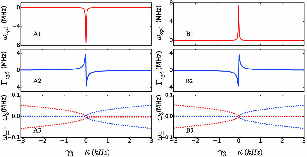
Fig. 2. Mechanical responses and the supermodes spectrum as a function of γ 3 . Frequency shifts are plotted in A1 and B1; A2 and B2 denote the optical damping rate Γ opt . Here the real and imaginary parts of complex numbers ω ± are denoted by the red and blue dashed lines, respectively. A1–A3 indicate the mechanical responses and supermode spectrum with blue-detuned driving. B1–B3 plot the mechanical responses and supermode spectrum in the red sideband driving regime. The parameters used are κ = 1 MHz , P in = 17.5 μ W , γ 2 = 2.6 MHz , g 0 = 4 Hz , Ω m = 50 MHz , Γ m = 1 kHz , J = κ , δ 3 = − 1.95 kHz , and δ 1 = 0.99 δ 3 .

Fig. 3. Absolute value of the mechanical frequency shift Δ Ω m ( ν ) and effective linewidth Γ ( ν ) with the perturbation ν . The red lines show the absolute value of the mechanical frequency shift and the blue dashed lines plot Γ ( ν ) in (a) and (b) with δ 1 = δ 3 = 5 kHz . The difference between A b s ( Δ Ω m ( ν ) ) and Γ ν are plotted in (c) and (d) with the detuning δ 3 and the perturbation ν . The coupling rates J are 0.97 κ and 1.01 κ in (c) and (d), respectively. Other parameters used here are γ 3 = 1 MHz , κ = 0.975 γ 3 , and Γ = 5 Hz .

Fig. 4. Cavity emission spectrum with the effect of laser frequency noise in (a) and (b). The perturbation ν equals 300 Hz and the mechanical linewidth is 1 Hz. The insets show the mechanical frequency shift induced by laser frequency noise σ . The coupling rate J = 0.8 κ in (a) and J = κ in (b). (c) We plot η as a function of σ with different coupling rates J . The red line indicates the system is robust to laser frequency noise near the exceptional point. The parameters used here are γ 3 = 1.00 MHz , Δ 1 = Ω m , Δ 3 = Ω m , κ = 0.985 γ 3 , and Γ = 1 Hz .

Fig. 5. (a) Normalized output spectra with different optical frequency shifts ν . The black solid line represents the cavity emission spectrum without external perturbation when the mechanical linewidth is 1 Hz. And the output spectrum is normalized to 1 separately. (b) The resolution of ν as a function of the coupling rate J . The red, green, and blue solid lines indicate the minimum detectable optical cavity resonance shift with Γ = 2 , 1, and 0.5 Hz, respectively. The parameters used here are γ 3 = 1.00 MHz , Δ 1 = Ω m , Δ 3 = Ω m , and κ = 0.985 γ 3 . And the coupling rate J = κ in (a).

Set citation alerts for the article
Please enter your email address