Driving a system periodically can generate new out-of-equilibrium phases that differ substantially from the original undriven system. Such driven phases are ubiquitous and have been extensively studied in physics, from Kapitza’s pendulum in mechanics [1] to Thouless pumping in quantum physics [2,3]. An important milestone for periodic driving was the discovery of dynamic localization (DL) in atomic physics in 1986 [4]. Naively, one might expect that applying a periodic force to a wave packet would cause it to accelerate or scatter. However, as the name suggests, in DL, one can drive a lattice containing a single electron in a way that suppresses the coupling between lattice sites, making them behave as if fully disconnected. This counterintuitive influence of DL has been observed in manifold experiments and is now understood to be a general wave phenomenon [5–18].

The past two decades have seen a surge of interest in Floquet engineering, which is a considerable extension of DL and encompasses a range of techniques to modify a wave system’s behavior using a periodic driving field. Experimentally, Floquet driving has been realized in manifold systems, from condensed matter [19–24], to cold atoms [25–32], to photonics [33–41]. Notably, the demonstration of Floquet topological insulators in curved waveguide arrays had a progenitive role in topological photonics [42–49]. The beauty of Floquet engineering lies in its simplicity: driving a system periodically gives us new degrees of control, allowing us to generate novel behaviors. At the same time, conventional Floquet engineering is also a rather blunt instrument, with only a few available parameters (driving strength, frequency, and in some cases polarization and polychromatic waves [50–55]), giving us limited leverage to induce a desired behavior in a prefabricated physical platform. So far, spatial degrees of freedom have been exploited in limited, specific contexts [21,56–59].

Here, we open up the full set of spatial degrees of freedom in Floquet engineering, giving us greater control over systems. Specifically, we show that with properly tailored driving fields, we can make a large class of 1D nearest-neighbor tight-binding Hamiltonians behave as any other, to a leading order in perturbation theory. This allows us to carry out applications previously thought impossible, such as undoing Anderson localization [60–70]; i.e., we show a tailored drive can turn a disordered system into an effectively ordered one. We also construct a spatially dependent driving that has the opposite effect, inducing Anderson localization in a regular lattice.

Space-time-dependent Floquet engineering is conceptually straightforward. Though our primary physical application in this paper is photonic waveguides, it is illustrative to begin with a more generic example. Consider an arbitrary physical system governed by the time-independent Hamiltonian $\mathcal{H}$. We wish to drive $\mathcal{H}$ with a space- and time-dependent field driving $F$ such that the overall system ${\mathcal{H}}^{\prime }$ behaves as a desired time-independent Hamiltonian ${\mathcal{H}}_{\mathrm{eff}}$. That is, $${\mathcal{H}}^{\prime }(\overrightarrow{x},t)=\mathcal{H}(\overrightarrow{x})+F(\overrightarrow{x},t)\sim {\mathcal{H}}_{\mathrm{eff}}(\overrightarrow{x}).$$(1)

The novel ingredient in this paper is that we allow $F$ to have not just time dependence but also spatial dependence. We give $F$ a time periodicity $T$ and frequency $\omega =2\pi /T$. Let us pause to emphasize that this work only explicitly considers monochromatic driving fields, whose spatial degrees of freedom will prove quite powerful. Combining this with further degrees of freedom like multiple frequencies on top of spatial dependencies can expand our reach yet further.

In theory, there may be an infinitely large number of $F$ we can choose in Eq. (1) that adequately approximate the behavior ${\mathcal{H}}_{\mathrm{eff}}$. In practice, however, the range of Hamiltonians $\mathcal{H}$ that we can fabricate and the fields $F$ we can create may be significantly limited by experimental capabilities. Our goal is to develop a straightforward recipe for engineering driving fields $F$ that approximately produce the desired behavior ${\mathcal{H}}_{\mathrm{eff}}$, subject to such experimental constraints.

Perturbation theory is one method to approximately solve Eq. (1), as the driving field frequency serves as a natural small expansion parameter. We can obtain a time-independent approximation of a driven system’s behavior using a Magnus expansion [71], a tool originally developed in the applied mathematics literature for solving a class of differential equations that naturally includes many time-periodic systems in physics; as such, it is used extensively in Floquet engineering across many physical platforms, e.g., Refs. [72–74]. Dropping spatial arguments $\overrightarrow{x}$ for concision, the Magnus expansion takes the form $$\begin{gathered} {\int }_0^T\mathrm{d}t{\mathcal{H}}_{\mathrm{eff}}={\int }_0^t\mathrm{d}{t}_1{\mathcal{H}}^{\prime }(t_1)+\frac{1}{2}{\int }_0^t\mathrm{d}{t}_1{\int }_0^{t_1}\mathrm{d}{t}_2[{\mathcal{H}}^{\prime }(t_1),{\mathcal{H}}^{\prime }(t_2)] \\ +\frac{1}{6}{\int }_0^t\mathrm{d}{t}_1{\int }_0^{t_1}\mathrm{d}{t}_2{\int }_0^{t_2}\mathrm{d}{t}_3\{[{\mathcal{H}}^{\prime }(t_1),[{\mathcal{H}}^{\prime }(t_2),{\mathcal{H}}^{\prime }(t_3)]]+[{\mathcal{H}}^{\prime }(t_3),[{\mathcal{H}}^{\prime }(t_2),{\mathcal{H}}^{\prime }(t_1)]]\}+\dots . \end{gathered}$$(2)

The left-hand side (LHS) of this equation evaluates to simply $T{\mathcal{H}}_{\mathrm{eff}}$, as ${\mathcal{H}}_{\mathrm{eff}}$ is time-independent. On the right-hand side (RHS), the $n$th order term consists of commutators nested $n$ times. The first term on the RHS is $\mathcal{O}({\omega }^0)$ and describes the dispersion that would occur if $F$ were averaged out. The second term on the RHS is an $\mathcal{O}({\omega }^{-1})$ correction. (In DL, these two terms are often treated collectively.) The first term on the RHS may depend on $F$ and differ from the undriven $\mathcal{H}$. While in principle the Magnus expansion has known convergence issues in various scenarios [72,75–77], we will see that, in practice, it can serve as a strong starting point for spatially nonuniform Floquet engineering.

Let us consider a simple illustrative example, taking the Hamiltonians’ Eq. (1) to have the form of a matrix, and imposing a sinusoidal driving $F(t)=F_0\sin (\omega t)$, with $F_0$ also a matrix. Evaluating Eq. (2) over one period of oscillation $T=2\pi /\omega$, we have $$\frac{2\pi }{\omega }{\mathcal{H}}_{\mathrm{eff}}\approx \frac{2\pi }{\omega }\mathcal{H}+\frac{2\pi }{{\omega }^2}[\mathcal{H},F_0]-\frac{3\pi }{2{\omega }^3}[F_0,[\mathcal{H},F_0]]+\mathcal{O}({\omega }^{-4}).$$(3)

Finding an appropriate driving field $F(t)$ that makes ${\mathcal{H}}_0$ behave as some new effective Hamiltonian ${\mathcal{H}}_{\mathrm{eff}}$ at $\mathcal{O}({\omega }^{-1})$ accuracy thus amounts to solving an inverse commutator problem, $${\mathcal{H}}_{\mathrm{eff}}-\mathcal{H}=\frac{1}{\omega }[\mathcal{H},F_0],$$(4)where the goal is to calculate $F_0$ in terms of $\mathcal{H}$ and ${\mathcal{H}}_{\mathrm{eff}}$. Note that while there are many choices of time-dependent driving fields, they typically reduce to an inverse commutator problem resembling Eq. (4). Solving Eq. (4) for $F_0$ is a straightforward algebraic exercise (see Appendix A). {Note that Eq. (4) defines the elements of a Lie algebra. For example, in the case of real $n\times n$ matrices, we have the general linear Lie algebra on the real numbers, $\mathfrak{g}{\mathfrak{l}}_n(\mathbb{R})$. Solutions then belong to the Eq. (4) subgroup, the special linear Lie algebra $\mathfrak{s}{\mathfrak{l}}_n(\mathbb{R})$. Properties of Lie algebras are well known, and restrict the form of what ${\mathcal{H}}_{\mathrm{eff}}$ in Eq. (4) we can achieve exactly; for example, taking the trace on both sides of Eq. (4), we see that $\mathcal{H}-{\mathcal{H}}_{\mathrm{eff}}$ must always be traceless. However, we remind the reader that here we are pursuing approximate solutions, and Eq. (4) is itself an expansion. It is straightforward to consider more general classes of operators as well, such as non-Hermitian systems [78–82].}

As a concrete implementation of space-time-dependent Floquet engineering, we consider an array of curved paraxial waveguides with low refractive index contrast. In the slowly varying envelope (paraxial) approximation, waves traveling through this system obey a Schrödinger-like equation, $$i{\partial }_z\psi (\overrightarrow{x},z)=\mathcal{H}\psi =\{\frac{i}{2k_0}{\nabla }^2-\frac{k_0}{r_0}[n(\overrightarrow{x},z)-n_0]\}\psi .$$(5)

Here, $\mathcal{H}$ is the Hamiltonian, $\psi$ is the wave function, $n(\overrightarrow{x},z)$ is the local distribution of the refractive index, and $k_0=2\pi n_0/\lambda$ is the wavenumber. The axis of wave propagation is $z$, which plays the same role as time $t$ in Section 2. The vector $\overrightarrow{x}$ signifies transverse directions. In the paraxial approximation, the array behaves like a tight-binding model. The curvature of the waveguides induces a $z$-dependent driving field $F(\overrightarrow{x},z)$.

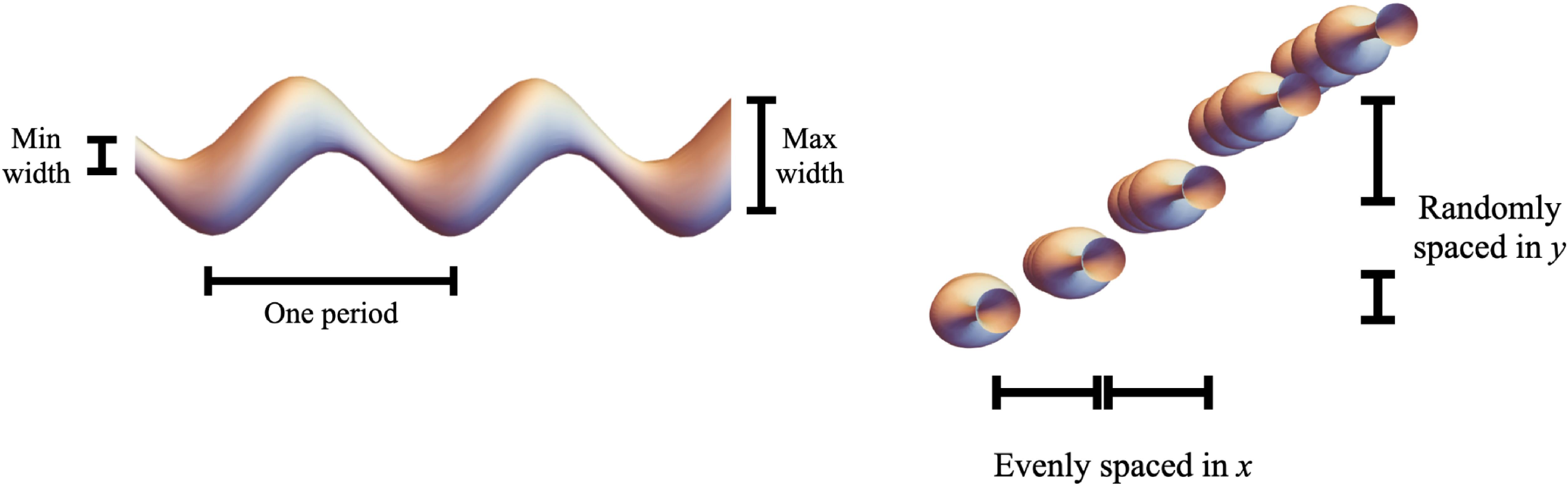
The simplest such system we can analyze occurs when the wave guides have only nearest-neighbor (nn) couplings. Straight (undriven) nn-coupled wave guides are described by a $z$-independent tridiagonal matrix, $${\mathcal{H}}_0=\gamma +{\gamma }^{†},$$(6)where ${\gamma }_{ij}={\gamma }_i{\delta }_{i+1,j}$ has nonzero entries only on the first off-diagonal describing the couplings. In the examples used in this paper, we take randomly chosen couplings, ${\gamma }_i\in [\mathrm{0.2,}1]$. To induce a driving field in this array, we curve the wave guides along zigzagged paths, as sketched in Fig. 1. Concurrently, we undulate the width of each wave guide periodically. The wave guides oscillate in unison, so their distances are $z$-independent. We make the wave guide trajectories locally parabolic, inducing an artificial gauge field on the wave packets and causing the nn couplings $\gamma$ to rotate phase as ${\gamma }_k\exp (\pm i\omega z)$. We vary the on-site potential $V$ and modulate the wave guide thickness as $\cos (\omega z)$, alternating sign $\pm$ after each period. The propagation of light through the driven system is governed by the $z$-dependent Hamiltonian, $${\mathcal{H}}_{\text{driven}}(z)=\gamma e^{i\omega z}+{\gamma }^{†}{e}^{-i\omega z}+V+\cos (\omega z),$$(7)as explained in greater detail in Appendices B and C.

Let us find the lowest-order effective Hamiltonian that describes the behavior of Eq. (7). Applying the Magnus expansion in Eqs. (2)–(7) and averaging over one period, we have $${\mathcal{H}}_{\mathrm{eff}}=V+\frac{1}{\omega }(2[\gamma ,{\gamma }^{†}]-[ϵ,\gamma -{\gamma }^{†}]+2[V,\gamma -{\gamma }^{†}])+\mathcal{O}({\omega }^{-2}).$$(8)Recall that the Schrödinger equation carries an extra factor of $-i$, which both lies in ${\mathcal{H}}_{\mathrm{eff}}$ and propagates throughout the Magnus expansion. The terms $V$ and $[\gamma ,{\gamma }^{†}]$ are both diagonal matrices. The other two commutators in Eq. (8) have nonzero elements only on their first off-diagonals.

Let us now curve the wave guides (i.e., by choosing appropriate $V$ and $ϵ$) such that ${\mathcal{H}}_{\mathrm{eff}}$ behaves approximately as some $z$-independent system, $${\mathcal{H}}_{\mathrm{eff}}=V_{\mathrm{eff}}+{\gamma }_{\mathrm{eff}}+{\gamma }_{\mathrm{eff}}^{†},$$(9)where $V_{\mathrm{eff}}$ is again diagonal and ${\gamma }_{\mathrm{eff}}$ has nonzero entries only on the first off-diagonal. We begin by equating the LHS of Eq. (8) with the LHS of Eq. (9), which simplifies to $$[ϵ,\gamma -{\gamma }^{†}]=(\omega V+2[\gamma ,{\gamma }^{†}]-\omega V_{\mathrm{eff}})+(2[V,\gamma -{\gamma }^{†}]-\omega {\gamma }_{\mathrm{eff}}-\omega {\gamma }_{\mathrm{eff}}^{†}).$$(10)

On the RHS, the first parenthetical set of terms is purely diagonal, and the second set of terms is purely off-diagonal. It is straightforward to check that the RHS is purely Hermitian. Likewise, on the LHS, $\gamma -{\gamma }^{†}$ is skew-Hermitian. Thus, $ϵ$ is Hermitian, i.e., ${ϵ}_{ij}={ϵ}_{ji}$.

We have enough degrees of freedom available that we can take $ϵ$ to be tridiagonal. In this case, let us examine the terms of the $ϵ$-commutator in Eq. (10), $${[ϵ,\gamma -{\gamma }^{†}]}_{ik}={\gamma }_{k-1}{ϵ}_{i,k-1}-{\gamma }_k{ϵ}_{i,k+1}-{\gamma }_i{ϵ}_{i+1,k}+{\gamma }_{i-1}{ϵ}_{i-1,k}.$$(11)

This commutator is also tridiagonal. We can examine each diagonal $k=i,i\pm 1$ separately, $$\begin{gathered} {[ϵ,\gamma -{\gamma }^{†}]}_{i,i+1}={\gamma }_i({ϵ}_{i,i}-{ϵ}_{i+1,i+1}), \\ {[ϵ,\gamma -{\gamma }^{†}]}_{ii}=2{\gamma }_{i-1}{ϵ}_{i,i-1}. \end{gathered}$$(12)Combining Eq. (12) with Eq. (10), we find that $$\begin{gathered} {ϵ}_{i-1,i}={ϵ}_{i,i-1}=\frac{1}{2{\gamma }_{i-1}}{(\omega V+2[\gamma ,{\gamma }^{†}]-\omega V_{\mathrm{eff}})}_{ii}, \\ {ϵ}_{i,i}-{ϵ}_{i+1,i+1}=\frac{1}{{\gamma }_i}{(2[V,\gamma -{\gamma }^{†}]-\omega {\gamma }_{\mathrm{eff}})}_{i,i+1}. \end{gathered}$$(13)

The latter equation allows us to construct the diagonal terms of $ϵ$ recursively, $${ϵ}_{ii}=\sum _{k=1}^i\frac{1}{{\gamma }_{n-i}}{(2[V,\gamma -{\gamma }^{†}]-\omega {\gamma }_{\mathrm{eff}})}_{n-i,n-i+1},$$(14)with ${ϵ}_{nn}=0$. Note that using this scheme, we still have additional degrees of freedom we can exploit; namely, we can alter the on-site potential $V$ to change the structure of $ϵ$.

The analytically tailored driving field (curvature) removes disorder up to $\mathcal{O}({\omega }^{-2})$ corrections. If we use large driving frequencies $\omega$, all terms of ${\mathcal{H}}_{\mathrm{eff}}$ are small, and thus the dynamics are slow and of small bandwidth. In many cases, it is possible to reduce the effect of $\mathcal{O}({\omega }^{-2})$ corrections without explicitly working at the next order in the expansion of $H_{\mathrm{eff}}$, by numerically optimizing the choice of $V$ and $ϵ$.

Here, let us take our desired Hamiltonian ${\mathcal{H}}_{\mathrm{eff}}$ to have uniform nearest-neighbor couplings ${\gamma }_{\mathrm{eff}}^{ij}=\mathrm{\Gamma }{\delta }^{i,j+1}$ and no on-site potential $V_{\mathrm{eff}}=0$.

Example 1.

Let us assume $V=0$. Then our driving field is $\cos (\omega z)$, and we can identify $$\begin{gathered} {ϵ}_{i-1,i}={ϵ}_{i,i-1}=\frac{1}{{\gamma }_{i-1}}({\gamma }_i^2-{\gamma }_{i-1}^2), \\ {ϵ}_{ii}=-\omega \mathrm{\Gamma }\sum _{k=1}^i\frac{1}{{\gamma }_{n-i}}. \end{gathered}$$(15)

Example 2.

We could also choose to work with both an on-site potential and a driving field $V+\cos (\omega z)$. In this case, it is possible to eliminate the off-diagonal terms in $ϵ$ by fixing $V$ properly. Specifically, we can take $$\begin{gathered} V_{ij}=-\frac{2}{\omega }{[\gamma ,{\gamma }^{†}]}_{ij}=-\frac{2}{\omega }({\gamma }_i^2-{\gamma }_{i-1}^2){\delta }_{ij}, \\ {ϵ}_{i,i\pm 1}=0, \\ {ϵ}_{ii}=\sum _{k=1}^i\frac{1}{{\gamma }_{n-i}}{(-\frac{4}{\omega }[[\gamma ,{\gamma }^{†}],\gamma -{\gamma }^{†}]-\omega \mathrm{\Gamma })}_{n-i,n-i+1}=-\omega \mathrm{\Gamma }\sum _{k=1}^i\frac{1}{{\gamma }_{n-i}}. \end{gathered}$$(16)

In Fig. 2(A), we show how waves propagate through a set of straight wave guides, as described by Eq. (6). These waveguides are disordered, so we expect Anderson localization to bring transverse transport in the array to a halt [83]. In Fig. 2(A), we see that a localized beam incident on the array does indeed remain localized.

In Fig. 2(B), we consider propagation through the wave guide when acted upon by a simple, spatially uniform AC driving field. This case corresponds to an $ϵ$ that is proportional to the site index, so that the difference between every two sites (the electric field) is constant. Whatever the field amplitude, we do not expect the localizing effect of disorder to be undone, so as an example we take the amplitude for which an equivalent ordered lattice would not undergo localization. As expected, an AC field generally causes a wave packet to diffuse and eventually arrests its propagation (except in extreme cases, like that when the field strength is so large as to completely dominate the Hamiltonian’s behavior and dwarf the disorder).

In Fig. 2(C), we construct one possible curvature of the wave guides (driving field) in Eq. (7) that counteracts the disorder in the wave guides, making the system behave as an effectively uniform, ordered array. To do so, we calculate appropriate choices of $V$ and $ϵ$ that produce the desired effective Hamiltonian. Specifically, we make a choice of $ϵ$ that is purely diagonal, as described in Section 3.A and Fig. 3. Note that to construct the driving field used in this figure, we first carry out calculations using the procedure outlined above, which we use as the starting point for a numerical optimization of diagonal matrices $V$ and $ϵ$ producing the desired behavior.

In Fig. 2(D), we show that in contrast, applying an arbitrary driving force typically results in diffusive behaviors. In some cases, time-dependent disorder can even lead to anomalous faster-than-ballistic diffusive transport [84]. For our curved wave guides, we also find diffusive behavior if the driving parameters are arbitrarily chosen. This is in sharp contrast with the elimination of disorder that appears when the spatial dependence of the drive is tailored according to our prescription. The elimination of disorder we can obtain by appropriately driving the system is therefore in sharp contrast with typical regime of periodically driven disorder.

We obtain these results for relatively low $\omega =6$ where higher-order correction terms cannot be outright neglected. [For a sense of scale, recall that the random couplings ${\gamma }_i$ are taken to be $\mathcal{O}(1)$.] Since the magnitude of ${\mathcal{H}}_{\mathrm{eff}}$ is proportional to ${\omega }^{-1}$, the dynamics of the driven system are comparable in speed to the dynamics of the undriven system, which is a clear advantage for experiments. Nevertheless, the influence of ${\omega }^{-2}$ effects is seen to be practically small, especially if further numerical optimization of the driving parameters is performed.

Another capability of our approach is the generalization of DL, as shown in Fig. 4. DL is typically only considered for spatially regular (periodic) lattices; it is commonly believed to fail in inhomogeneous lattices, with the notable exception of driven Glauber–Fock lattices [85]. The situation changes remarkably if we use a spatially inhomogeneous driving: it is clear from our explorations of Eqs. (2) and (7) that an appropriately tailored driving field could induce DL even in a lattice that is completely irregular. This gives us the powerful ability to sever specific links and effectively cut out parts of a lattice by driving it with an appropriate spatially inhomogeneous field. For example, we could create an artificial sharp edge in a topological system, such as in Refs. [25,27] and expect to see edge modes there. This technique extends to complicated, highly nonuniform, and even multidimensional lattices, which all obey a operator form similar to Eq. (2).

Floquet engineering has of course seen extensive applications beyond the curved wave guides we have examined here. For example, we could study different physical platforms, alternative methods of implementing a driving field, or even tinker with additional degrees of freedom such as frequencies. Spatially nonuniform Floquet engineering techniques can straightforwardly be applied to these systems as well. When constructing a spatially nonuniform Floquet driving field in any given case, one must strike a delicate balance between challenges in the mathematical calculation and physical implementation.

When using perturbative methods to design a driving field, the nature of the Magnus expansion places restrictions on the Hamiltonians and driving fields. For example, to solve Eq. (2) at $\mathcal{O}({\omega }^{-1})$, we generally must solve an inverse commutator problem of the form ${\mathcal{H}}_{\mathrm{eff}}=[{\mathcal{H}}_0,F]$. If ${\mathcal{H}}_{\mathrm{eff}}$ and ${\mathcal{H}}_0$ are both Hermitian, then $F$ must be skew-Hermitian. Likewise, if ${\mathcal{H}}_{\mathrm{eff}}$ and $F$ are Hermitian, then ${\mathcal{H}}_0$ is skew-Hermitian. Skew-Hermitian wave guide schemes or driving fields may be difficult to fabricate. This does not, however, render Magnus expansion methods impracticable. Indeed, our curved wave guide setup satisfied the skew-Hermitian criterion, and other potential implementations exist.

Alternatively, one could circumvent the problem of skew-Hermiticity by choosing a driving field $F$ such that the $\mathcal{O}({\omega }^{-1})$ term $[{\mathcal{H}}_0,F]$ vanishes and the leading term in the Magnus expansion is an $\mathcal{O}({\omega }^{-2})$ integral over the double-commutator $[F,[{\mathcal{H}}_0,F]]$. In this case, ${\mathcal{H}}_{\mathrm{eff}}$, ${\mathcal{H}}_0$, and $F$ can be Hermitian simultaneously. However, even if ${\mathcal{H}}_{\mathrm{eff}}$ and ${\mathcal{H}}_0$ are tridiagonal, $F$ may have nonzero terms on its second off-diagonal (or vice versa). This has its own set of challenges for experimental realization.

The leading-order Magnus expansion provides a straightforward demonstration of the power of space-time-dependent Floquet engineering. However, a naive Magnus expansion is not optimal for solving high-precision Floquet engineering problems at low computational cost, and more creative approaches are necessary to fully capitalize on the power of space-time modulations, within physical constraints. For example, one could consider alternative approximation schemes (see, e.g., Ref. [86]) or simply use numerical optimization to determine a spatially nonuniform driving field that produces as close to the desired behaviors as possible. The potential for harnessing the full power of space-time Floquet engineering for physical applications is bright.

We open up Floquet engineering to the full breadth of space-time-dependent driving fields, giving us greater control over wave systems. By exploiting spatial degrees of freedom, we showed that we could both induce DL in nonuniform lattices and undo Anderson localization by giving photonic wave guides appropriate curvature. The technique is more broadly applicable, and we foresee its use in a range of atomic, optical, and condensed matter systems. In the future, perhaps this technique can help in fabricating classes of Hamiltonians that currently are difficult or implausible to realize, such as imaginary gauge fields, Hamiltonians with only next-nearest-neighbor couplings, or non-Abelian Hamiltonians.

Acknowledgment. We thank Mordechai Segev and Yaakov Lumer for initial work on this project many years past [87], and S. T. S. is grateful to Moti for hosting her as a summer research student during that time. We thank Momchil Minkov and Pengning Chao for interesting discussions.