 AI Video Guide
  AI Picture Guide
 AI One Sentence

Zheng Huang, Conghe Wang, Caihua Zhang, Wanxin Shi, Shukai Wu, Sigang Yang, Hongwei Chen, "Brain-like training of a pre-sensor optical neural network with a backpropagation-free algorithm," Photonics Res. 13, 915 (2025)
- Photonics Research
- Vol. 13, Issue 4, 915 (2025)
Note: This section is automatically generated by AI . The website and platform operators shall not be liable for any commercial or legal consequences arising from your use of AI generated content on this website. Please be aware of this.
Abstract
1. INTRODUCTION
Deep learning models, like convolutional neural networks (CNNs) [1], recurrent neural networks (RNNs) [2], and transformers [3], have emerged as pervasive instruments within the realms of science and engineering, facilitating the accomplishment of diverse and intricate tasks. Nevertheless, traditional electronic computing hardware grapples with challenges like the breakdown of Moore’s Law and heightened power consumption, presenting obstacles in meeting the escalating demand for computational power. Deep physical neural networks capitalize on specific physical carriers, such as light, as computing media. This paradigm relocates the mathematical computation process, originally confined to the digital domain, to physical hardware, showcasing notable advantages in speed, power efficiency, and throughput.
Optical neural networks (ONNs) [4–6] are being rigorously investigated for their potential to accelerate computations in deep learning efficiently, attributed to the characteristics of high speed, broad bandwidth, and low power consumption. Various ONN implementations modulate the amplitude, phase, and polarization of light by optical elements such as metasurfaces and spatial light modulators (SLMs) [7–18], executing linear computations in free space. Nevertheless, the advent of next-generation applications such as autonomous driving and augmented reality (AR) necessitates a high response speed and superior energy efficiency to facilitate real-time decision-making in edge devices. To this end, pre-sensor optical computing has been proposed to offload substantial computational tasks from electronics into optics [19], thereby harnessing the inherent advantages of optical systems, where three keys must be met to make it feasible. Firstly, the pre-sensor processor must be capable of handling incoherent light illumination in real-world scenarios, processing the incoming information, and performing specific computations during light propagation. This processor should be integrated seamlessly with the mature machine vision pipeline, effectively replacing traditional imaging procedures. Secondly, the imperative for nonlinear activation between layers in ONNs remains, and optical-to-optical nonlinear activation could extend the layer depth and computational capabilities of ONNs. Thirdly, the design of optical elements, such as the patterns on an SLM or the specifications of silicon cylinders in the metasurface, must be optimized to ensure best performance [20,21].
To date, the predominant methodology for training ONNs has been the backpropagation (BP) algorithm [22,23], which has led to the emergence of three distinct paradigms: in-silico training, in-situ training, and combined training, as depicted in Fig. 1(b). The in-silico training approach involves creating a mathematical dual to the physical system. Model parameters are optimized through gradient descent, derived using the chain rule, thus enabling updates to the corresponding parameters of the optical system. A precise and differentiable mathematical representation is indispensable for the backward pass within the complete end-to-end training framework. In-situ training [24–26] entails direct physical computation and updates of the physical structure parameters on the device itself, leveraging the product approximation of the forward propagation and backpropagation results as a partial derivative of the applied loss function with respect to the weight values. This approach mitigates specific errors, such as those arising from fabrication discrepancies and the divergence between the mathematical digital model and the physical model. Nonetheless, the in-situ method entails performing both training and inference on the devices, which escalates hardware costs. The combined training [27–34] approach aims to balance training accuracy against hardware expenditures. For example, the physics-aware training method is proposed as a hybrid in-situ-in-silico method [27]. Here, the forward pass is conducted physically, while the backward pass is executed in-silico using a digital model that simulates the input-output transformations. This model is refined through extensive data training. Such dual training methodologies are also employed to design hardware parameters or rectify hardware-induced errors.
Sign up for Photonics Research TOC. Get the latest issue of Photonics Research delivered right to you!Sign up now
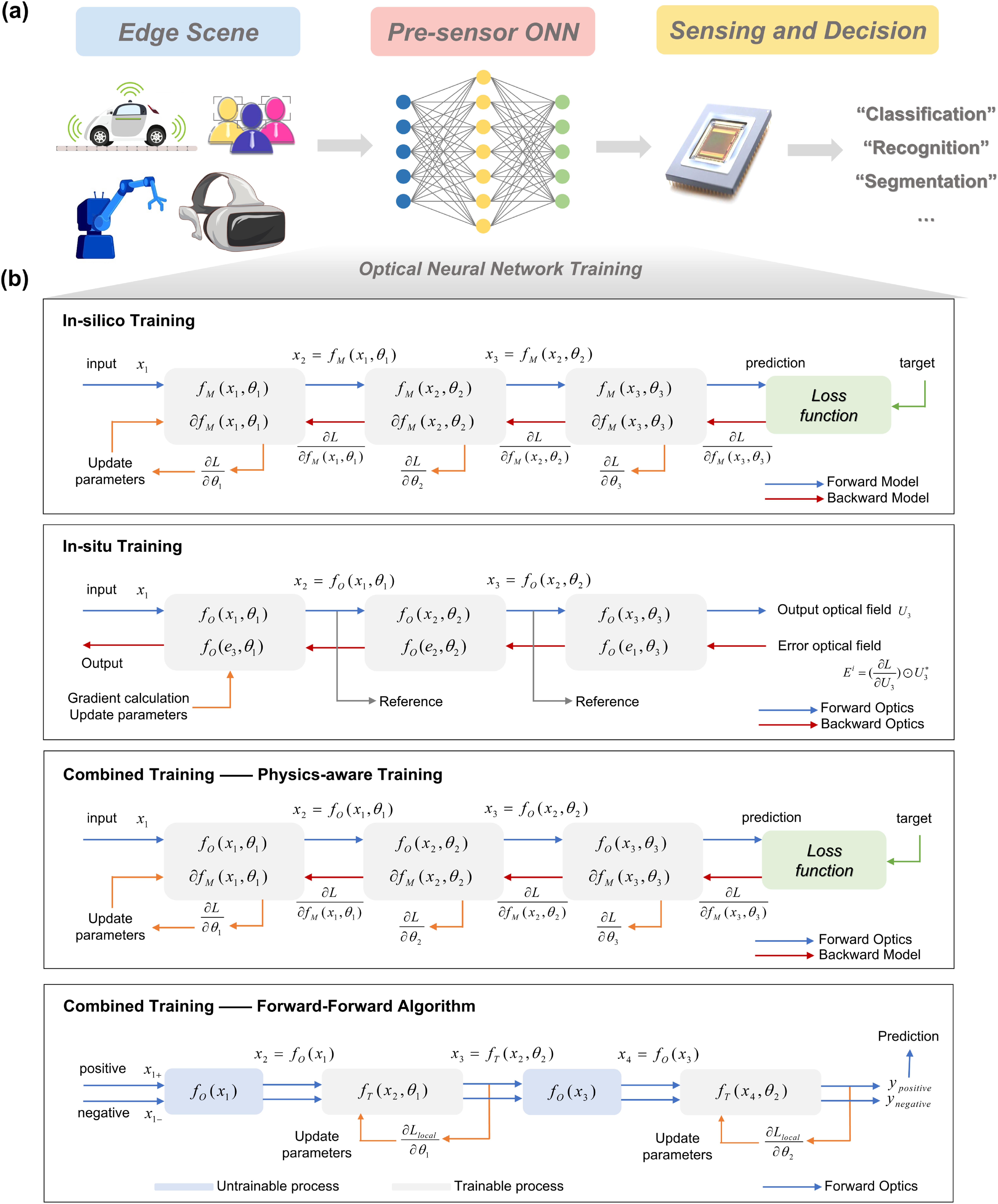
Figure 1.Paradigms for training ONNs:
However, the training algorithm based on BP possesses inherent limitations, especially the requirement that the physical process or its digital counterpart in forward propagation be differentiable. If a black box, whose operational principles and mathematical representation are undisclosed, is integrated into the forward propagation pathway, the BP-based training is predisposed to failure. Concurrently, to more closely mimic the training mechanisms of the human brain, ONNs can adapt to processing and learning from transmission data across different stages in real-time rather than relying solely on executing the BP process after data propagation. The forward-forward algorithm (FFA) is a local learning method that defines a local loss function within a segment of a model. Similar to reservoir computing, where the hidden layer is randomly initialized and remains fixed, the output layer serves as the sole trainable component, optimized through localized adjustments [35–40]. FFA is utilized in training physical neural networks; however, its application is primarily targeted towards digital linear layers rather than the physical parameters themselves, limiting the broader applicability of the FFA in diverse training contexts where adjustments to physical parameters are necessary.
In this paper, we demonstrate a pre-sensor optical computing system employing FFA to train both optical and digital parameters directly, analogous to the learning processes in the human brain. The optical component comprises a passive amplitude mask, an image intensifier, and an SLM, which facilitate nonlinear activation and linear modulation. Utilizing the training method of FFA, it becomes possible to train the optical linear segments and the corresponding digital linear components independently of understanding the nonlinear modulation processes executed by the image intensifier, enhancing the overall efficiency and adaptability of the system. The experimental results reveal an accuracy of 93% in the classification of the MNIST dataset using a single-layer ONN and an accuracy of 87.5% in the classification of the Fashion-MNIST dataset using a double-layer ONN. Broadly, the training method offers a promising approach to automatically design parameters for functional optical devices, particularly when certain components of the system cannot be explicitly modeled, empowering scenarios for pre-sensor optical computing with high speed, high efficiency, and low power consumption.
2. FORWARD-FORWARD ALGORITHM
The FFA was initially devised to address the lack of precise details in forward computation [41]. In this method, the conventional backward pass of backpropagation is replaced with a layer-specific local loss function, referred to as the “goodness function.” By presenting both positive and negative samples to each layer of the network, the objective of the goodness function is to ensure that the goodness for positive samples significantly exceeds that for negative samples, thereby classifying the input data as positive or negative. During the positive pass, data with the correct label are processed through forward propagation, with the weights adjusted to increase the goodness of the trainable layer. Conversely, during the negative pass, data with incorrect labels undergo the same forward propagation. Specifically, the parameters are optimized for each trainable layer by minimizing the following loss function:
The local loss function is designed to maximize the margin between positive and negative samples in the feature space, effectively promoting numerical stability for robust optimization.
3. NONLINEAR OPTICAL ACTIVATION FUNCTION OF IMAGE INTENSIFIER
Similar to the transmission rules of human neurons, which transmit signals only under specific stimuli, the activation function in neural networks acts as a control valve that regulates neuron activity. Nonlinear activation is crucial for neural networks to represent more complex functions. Without nonlinear activation functions between layers, all hidden layers lose their original purpose, as multiple layers of linear operations are equivalent to a single layer of linear operations. For ONNs, there are numerous methods to construct linear operations that lack nonlinear activation. Researchers have been exploring various approaches to achieve all-optical interlayer nonlinearity, such as using phase change materials [42], saturable absorbers [43,44], graphene materials [45], and quantum dots [19,46,47]. Two-dimensional (2D) spatial nonlinearity is particularly suitable for integration between two optical layers, providing stable and consistent nonlinearity. Recently, Wang
4. ONNS WITH TRAINING OF FFA FOR APPLICATIONS
A. Optimization of the Trainable Weights in ONNs
The training schematic is illustrated in Fig. 2(a). The entire process consists of two components: the black boxes, representing the optical process without a mathematical dual, and the trainable parts, which can be either optical or digital processes. The weights in the trainable parts are updated based on the local loss. Each input sample is embedded with a correct or incorrect label, corresponding to positive or negative data, respectively. The method for constructing data is depicted in Fig. 2(b). White squares are added to the four corners of a sample, representing binary values from 0001 to 0101 (decimal values from 1 to 10), which correspond to the digits from 0 to 9. The 4-bit binary range, spanning from 0000 to 1111, accommodates up to 16 distinct classes. This approach enhances the labeling capacity within a constrained marking area.
![]()
Figure 2.Optimization of the ONNs. (a) The schematic of the training process with FFA. (b) The method for constructing positive and negative samples, using handwritten numbers as an example.
B. Experiments for Machine Vision Tasks
We assessed the effectiveness of the proposed approach by developing a pre-sensor ONN for the task of classifying handwritten digits from the MNIST [48,49] dataset. The experimental setup is shown in Fig. 3(a). The samples are displayed on an LCD screen positioned approximately 15 cm away from the ONN encoder. In the pre-sensor ONN, an amplitude mask with a fixed pattern is placed in front of the image intensifier, which performs a convolution operation and extracts features from the input scene. The process of convolution in the optical domain is based on the principles of geometric optics, performing parts of the computing function [16]. The image intensifier then conducts an optical-to-optical nonlinear activation. An SLM (HOLOEYE LC2012) is positioned at the image plane of the image intensifier (S20 photocathode, IIM-C225 MCP, P46 phosphor screen), serving as a linear amplitude modulation via the Hadamard product. The sensor (Sony IMX 264) is positioned snugly against the SLM. In this configuration, the entire system comprising the mask and the image intensifier is treated as a black box. Due to the fixed pattern of the mask and the difficulty in accurately modeling the nonlinear activation function, these components are considered non-trainable and collectively regarded as a black box. The pattern in the SLM and the weights of the linear layers in the digital neural network are optimized using the FFA.
![]()
Figure 3.(a) Prototype of the system. (b) Corresponding network structure diagram of the system. (c) Confusion matrix in the classification of MNIST dataset, for the condition that only black box exists in the pre-sensor processing. (d) Confusion matrix in the classification of MNIST dataset, for the condition that black box and SLM coexist in the pre-sensor processing. (e) The optimized pattern of SLM. (f) The visualization of the output after black box. The samples represent the result of the convolutional layer formed by the mask and the nonlinear layer provided by the image intensifier. (g) Accuracy and parameters comparison across different models. The output neurons of the digital linear layer vary from 16 to 24. (h) The performances for the classification of CIFAR-4 dataset. The processing approaches contain only digital computing and the combination of optical and digital computing. (i) The optical nonlinear response of the image intensifier used in the experiments.
When measuring the nonlinear response of the image intensifier, the output light intensity is recorded as the input intensity varies. Figure 3(i) illustrates the relationship between the normalized input and normalized output of one output region in the image intensifier. Referring to Ref. [18], a four-parameter curve can be fit to the measured data pairs. However, the equation for the nonlinear activation curve is derived based solely on empirical observations, assuming its mathematical representation in advance. The nonlinear response can vary and be uneven among different neurons in the MCP, which leads to errors from inaccurate fitting and inconsistent nonlinearity. Moreover, the nonlinear curve is measured using power values, creating a gap between the actual physical and digital quantities when the nonlinear representation is used between layers in the end-to-end optimization of ONNs. Consequently, we can optimize the trainable weights in ONNs using the FFA without knowing the detailed properties of the nonlinear layer or training a digital twin model of it.
The input images from the MNIST dataset, originally at a resolution of
The performances for the classification of the MNIST dataset are presented in Table 1. The fully digital network employing BP and FFA achieved accuracies of 89.0% and 88.5% as the baseline. The integration of the black box enhanced the performance by 4%, reaching an accuracy of 92.5%, thereby underscoring the importance of linear and nonlinear modulation in optical processing. Following the capture post-black box, we optimized the weights in the element-wise Hadamard product layer, as well as the amplitude pattern of the SLM, as illustrated in Fig. 3(e). The incorporation of a linear layer, implemented through the SLM, further improved performance by 1.5% in the simulation and by 0.5% in the experiment, with the corresponding confusion matrices shown in Figs. 3(c) and 3(d). The performances of nonlinear optical processing and linear digital processing in classifying the MNIST dataset with varying output neuron counts are presented in Fig. 3(g). As the number of output neurons increases from 16 to 20, the classification accuracy improves steadily. However, beyond 20 output neurons, the rate of accuracy improvement diminishes. Meanwhile, the number of parameters and computational load continue to grow linearly with the increase in output neurons. Considering the trade-off between performance and computational efficiency, the number of output neurons is set to 20.
Comparison of Accuracies between Different Processing Approaches in the Classification of the MNIST Dataset
| Processing | Test Accuracy | Network (FC) | FLOPs |
|---|---|---|---|
| FC-BP | 89.0% | (784,22,10) | 3.5 × 10⁴ |
| FC-FFA | 88.5% | (1024,20) | 4.1 × 10⁴ |
| Black Box (optics) + FC-FFA | 92.5% | (900,20) | 3.6 × 10⁴ |
| Black Box (optics) + Linear (optics) + FC-FFA-sim | 94.0% | (900,20) | 3.6 × 10⁴ |
| Black Box (optics) + Linear (optics) + FC-FFA-exp | 93.0% | (900,20) | 3.6 × 10⁴ |
To further verify the role of linear and nonlinear modulation in the optical black box, we conducted experiments on the CIFAR-4 dataset [50,51], which contains four classes of “dog”, “frog”, “horse”, and “ship”. Initially, the RGB images with three channels were converted to grayscale. These grayscale images were directly connected to a fully connected linear layer (1024-20), whose weights were optimized using the FFA loss function. The results are shown in Fig. 3(h). The baseline classification accuracy for CIFAR-4 was 60.0%. After processing by an optical encoder, it yielded a classification accuracy of 67.5% for CIFAR-4, demonstrating that the optical black box improved task accuracy by 7.5%. It proves the function of pre-sensor optical computing.
We then performed the classification of the Fashion MNIST [52,53] dataset to evaluate the performance of the multilayer ONN encoder. The experimental setup closely mirrors that used for the classification of the MNIST dataset. The schematic diagram and corresponding network structure are shown in Figs. 4(a) and 4(b). The output of the optical processors, encompassing both nonlinear and linear components, is displayed on the LCD screen, resulting in an additional pre-sensor processing step in the optical domain. Consequently, the input images of fashion categories are processed sequentially through the black box and SLM in two cycles. It can also be realized by sequential placement of image intensifiers, SLM, and even other modulator components. Continuous linear and nonlinear transformations are performed with comprehensive feature extraction.
![]()
Figure 4.Experiments for Fashion MNIST dataset. (a) Schematic diagram of the system. The input includes positive and negative samples. (b) Corresponding network structure diagram of the system. “LM” means “linear modulation.” (c) The optimized pattern of SLM in the first optical linear layer of the Hadamard product. (d) The optimized pattern of SLM in the second optical linear layer of Hadamard product. (e) Confusion matrix in the classification of Fashion MNIST dataset, for the condition that the input images are processed sequentially through the black box and SLM in two cycles.
The data preparation method for constructing positive and negative samples for the Fashion MNIST dataset is the same as that for the MNIST dataset. The comparison of classification accuracies with different processing approaches is presented in Table 2. As a benchmark, we trained the digital fully connected layer using BP and FFA, achieving accuracies of 81.0% and 78.5%, respectively. When the amplitude mask and image intensifier were added to the optical path for pre-sensor computing, the accuracy improved by 1.5%, reaching 80.0%. We then co-trained the weights of the element-wise Hadamard product layer and the fully connected layer with FFA, achieving an accuracy of 86.0%. With the addition of further nonlinear and linear processing in the optical path, accuracies improved to 87.0% and 87.5%. Optical pre-sensor computing, which includes both linear and nonlinear components, improved accuracy by 9% while maintaining similar floating point operations (FLOPs) in the electronics.
Comparison of Accuracies between Different Processing Approaches in the Classification of Fashion MNIST Dataset
| Processing | Test Accuracy | Network (FC) | FLOPs |
|---|---|---|---|
| FC-BP | 81.0% | (784,22,10) | 3.5 × 10⁴ |
| FC-FFA | 78.5% | (1024,20) | 4.1 × 10⁴ |
| Black Box (optics) + FC-FFA | 80.0% | (900,20) | 3.6 × 10⁴ |
| Black Box (optics) + Linear (optics) + FC-FFA | 86.0% | (900,20) | 3.6 × 10⁴ |
| Black Box (optics) + Linear (optics) + Black Box (optics) + FC-FFA | 87.0% | (900,20) | 3.6 × 10⁴ |
| Black Box (optics) + Linear (optics) + Black Box (optics) + Linear (optics) + FC-FFA | 87.5% | (900,20) | 3.6 × 10⁴ |
In the classification of the Fashion MNIST dataset, we utilized a loop structure on the hardware to represent the effect of multiple optical computations. Due to the alternation of non-modellable linear layers with optimizable linear layers, the parameters of the linear layers can only be optimized using FFA. This method can also accommodate other nonlinear physical layers without requiring detailed knowledge of light propagation, enhancing the robustness of the optoelectronic system. Compared to the method of first fitting the parts lacking mathematical dual expressions with deep neural networks and then optimizing with BP, FFA enhances the efficiency of the training and reduces memory consumption by isolating the weight updates for individual layers.
5. DISCUSSION AND CONCLUSION
In this paper, we propose a pre-sensor multilayer ONN with nonlinear activation, trained using a brain-inspired learning algorithm, FFA. This approach is employed for training ONNs in situations where complete knowledge of the physical processes in the forward pass is unavailable, such as unknown or immeasurable nonlinearities during propagation. In the hardware system, a multilayer ONN is constructed with optimizable linear components and immeasurable nonlinear components. Compared to other ONN training methods, our approach eliminates the need to measure and fit nonlinear curves or to model input-output relationships with deep learning models, resulting in increased training accuracy and reduced computational costs. In the classification of the MNIST and Fashion MNIST datasets, the accuracies were improved by 4.5% and 9.0%, respectively, due to the addition of optical processing.
The current processing framework integrates pre-sensor computing within the optical domain and post-sensor processing in the electrical domain. Notably, the construction of all-optical neural networks using optical components is both feasible and promising. Convolution leverages the optical principles of spatial geometry, using passive masks or SLM, while the fully connected layer can be implemented through a combination of lenses and LCD modulators. These ONNs can facilitate linear and nonlinear modulation while allowing for training through backpropagation-free methodologies. For nonlinear activation between layers, the nonlinear methods employed in this study enhance the performance of classification tasks. However, the experimental results indicate that the improvement achieved through optical nonlinear activation is indeed limited. Unlike digital deep neural networks, where nonlinear activation functions can be designed arbitrarily, optical nonlinearity is primarily constrained by the inherent properties of the nonlinear materials employed. As a result, the performance gains from nonlinear components in optical systems may differ significantly from those observed in digital systems with mature nonlinear functions such as the “ReLU”. Furthermore, additional approaches to optical nonlinearity, such as quantum dots and photonic crystals, are being explored, which are expected to achieve customized optical nonlinear activation and reduce both power consumption and delay in decision-making with passive materials [19,46,47]. Thus, pre-sensor optical computing can offload part of the computation from electronics into optics by leveraging passive optical elements, further highlighting the advantages such as low power consumption, high speed, and high practicability, easily coupled with mature machine vision systems in edge computing.
6. MATERIALS AND METHODS
A. Mask Fabrication
The optical elements employed for pre-sensor computing in the experiment include an amplitude mask, an image intensifier, and an SLM. The mask utilized was created using photolithography methods on glass substrates coated with chromium. This fabrication process comprised multiple stages, including photolithography, development, etching, and demolding. The specific dimensions of the mask were chosen based on factors such as diffraction and geometric blurring. For our experiment, the feature size of the mask was established at 50 μm.
B. Dataset Processing and Neural Network Training
In our experiment, we utilized two standard classification datasets: the MNIST dataset and the Fashion MNIST dataset. We randomly selected a subset of 800 training images and 200 testing images for each dataset, with each class containing 80 training images and 20 testing images. These images were expanded into positive and negative samples. For training, each class had 80 positive samples and 720 negative samples. For testing, each class had 200 samples to evaluate.
The network training was conducted using PyTorch 1.13.1. During training, the Adam optimizer was employed with a learning rate set at 0.05 for the first 500 epochs and then adjusted to 0.008 for the last 500 epochs. The parameters were optimized by minimizing the local loss, as described in Section 2. All training operations were executed on a workstation equipped with an NVIDIA GeForce RTX 3090 GPU.
References
[1] K. O’shea, R. Nash. An introduction to convolutional neural networks. arXiv(2015).
[3] N. Parmar, A. Vaswani, J. Uszkoreit. Image transformer. International Conference on Machine Learning(2018).
[4] X. Sui, Q. Wu, J. Liu. A review of optical neural networks. IEEE Access, 8, 70773-70783(2020).
[22] R. Rojas, R. Rojas. The backpropagation algorithm. Neural Networks: A Systematic Introduction, 149-182(1996).
[41] G. Hinton. The forward-forward algorithm: some preliminary investigations. arXiv(2022).
[49] https://yann.lecun.com/exdb/mnist/. https://yann.lecun.com/exdb/mnist/
[50] A. Krizhevsky, G. Hinton. Learning multiple layers of features from tiny images, 7(2009).
[51] https://www.cs.toronto.edu/~kriz/cifar.html. https://www.cs.toronto.edu/~kriz/cifar.html


Set citation alerts for the article
Please enter your email address

© Copyright 2018-2021 | Chinese Laser Press. All Rights Reserved 沪ICP备15018463号-20