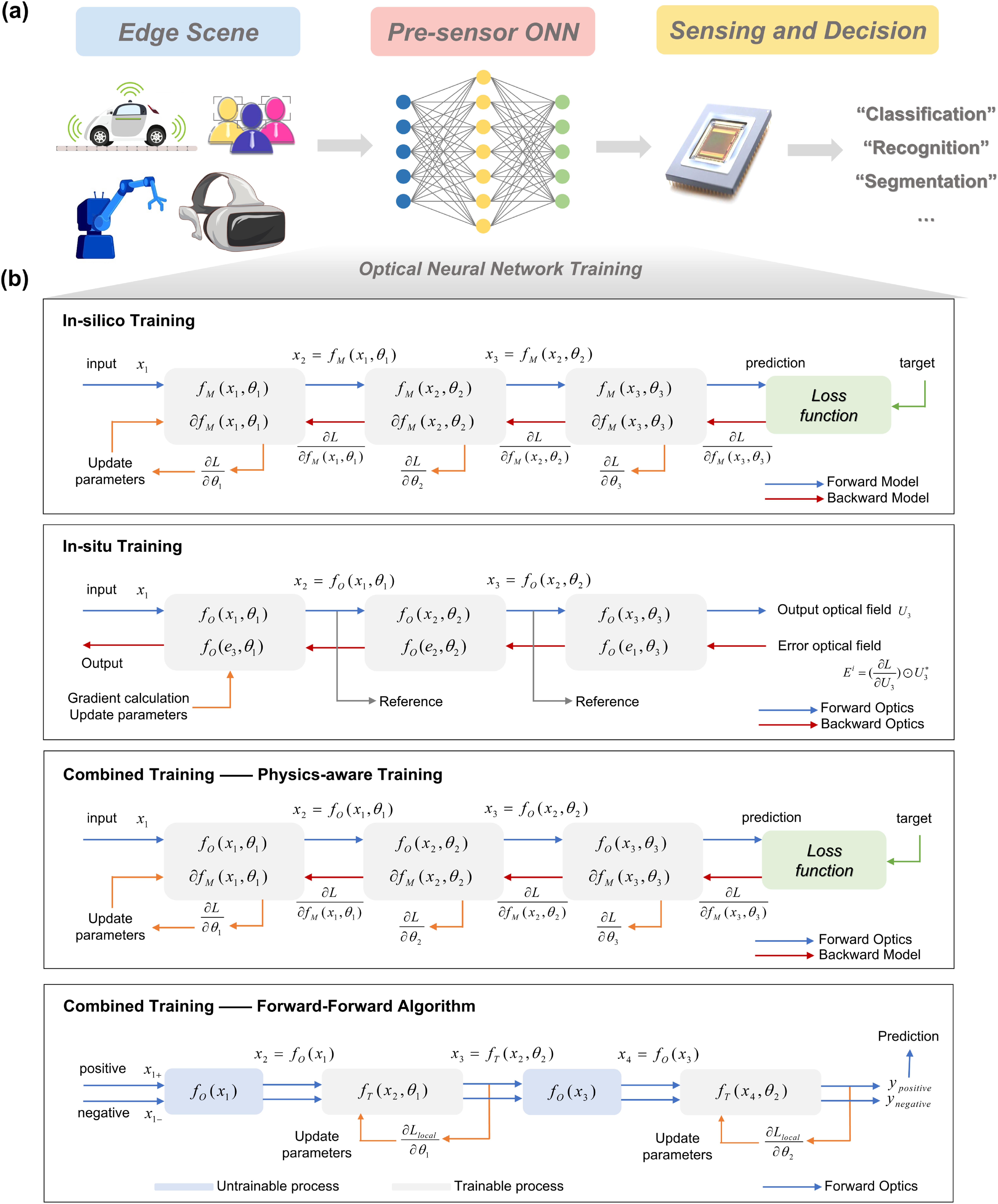
Fig. 1. Paradigms for training ONNs: in-silico training, in-situ training, combined training.

Fig. 2. Optimization of the ONNs. (a) The schematic of the training process with FFA. (b) The method for constructing positive and negative samples, using handwritten numbers as an example.

Fig. 3. (a) Prototype of the system. (b) Corresponding network structure diagram of the system. (c) Confusion matrix in the classification of MNIST dataset, for the condition that only black box exists in the pre-sensor processing. (d) Confusion matrix in the classification of MNIST dataset, for the condition that black box and SLM coexist in the pre-sensor processing. (e) The optimized pattern of SLM. (f) The visualization of the output after black box. The samples represent the result of the convolutional layer formed by the mask and the nonlinear layer provided by the image intensifier. (g) Accuracy and parameters comparison across different models. The output neurons of the digital linear layer vary from 16 to 24. (h) The performances for the classification of CIFAR-4 dataset. The processing approaches contain only digital computing and the combination of optical and digital computing. (i) The optical nonlinear response of the image intensifier used in the experiments.

Fig. 4. Experiments for Fashion MNIST dataset. (a) Schematic diagram of the system. The input includes positive and negative samples. (b) Corresponding network structure diagram of the system. “LM” means “linear modulation.” (c) The optimized pattern of SLM in the first optical linear layer of the Hadamard product. (d) The optimized pattern of SLM in the second optical linear layer of Hadamard product. (e) Confusion matrix in the classification of Fashion MNIST dataset, for the condition that the input images are processed sequentially through the black box and SLM in two cycles.

Table 1. Comparison of Accuracies between Different Processing Approaches in the Classification of the MNIST Dataset

Table 2. Comparison of Accuracies between Different Processing Approaches in the Classification of Fashion MNIST Dataset