Infrared and Visible Image Fusion Based on Structure-Texture Decomposition and VGG Deep Networks

Feiyan Yang; Meng Wang

doi:10.3788/LOP212808

Journals >Laser & Optoelectronics Progress >Volume 60 >Issue 2 >Page 0210008 > Article

Laser & Optoelectronics Progress
Vol. 60, Issue 2, 0210008 (2023)

Infrared and Visible Image Fusion Based on Structure-Texture Decomposition and VGG Deep Networks

Feiyan Yang^1,2 and Meng Wang^1,2,*

Author Affiliations

¹Faculty of Information Engineering and Automation, Kunming University of Science and Technology, Kunming 650500, Yunan, China

²Key Laboratory of Artificial Intelligence in Yunnan Province, Kunming 650500, Yunan, China

show less

DOI: 10.3788/LOP212808 Cite this Article Set citation alerts

Feiyan Yang, Meng Wang. Infrared and Visible Image Fusion Based on Structure-Texture Decomposition and VGG Deep Networks[J]. Laser & Optoelectronics Progress, 2023, 60(2): 0210008 Copy Citation Text

show less

Fig. 1. Framework of proposed method

Download full size

Example diagram of triband decomposition. (a) Input images; (b) high-frequency subbands; (c) low-frequency subbands; (d) low-frequency structures; (e) low-frequency textures

Fig. 2. Example diagram of triband decomposition. (a) Input images; (b) high-frequency subbands; (c) low-frequency subbands; (d) low-frequency structures; (e) low-frequency textures

Download full size

Fig. 3. Flow chart of high-frequency subband fusion

Download full size

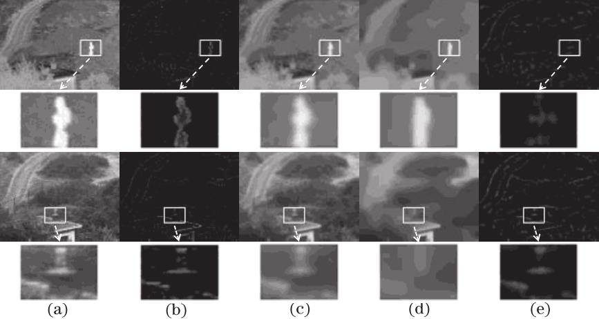
Fig. 4. Fusion results of “Camp” source image. (a) Infrared images; (b) visible image; (c) CBF; (d) JSR; (e) JSRSD; (f) DRTV; (g) CVT-SR; (h) GTF; (i) MISF; (j) proposed method

Download full size

Fig. 5. Fusion results of “Street” source image. (a) Infrared images; (b) visible image; (c) CBF; (d) JSR; (e) JSRSD; (f) DRTV; (g) CVT-SR; (h) GTF; (i) MISF; (j) proposed method

Download full size

Fig. 6. Fusion results of “Gate” source image. (a) Infrared images; (b) visible image; (c) CBF; (d) JSR; (e) JSRSD; (f) DRTV; (g) CVT-SR; (h) GTF; (i) MISF; (j) proposed method

Download full size

Fig. 7. Fusion results of “Car” source image. (a) Infrared images; (b) visible image; (c) CBF; (d) JSR; (e) JSRSD; (f) DRTV; (g) CVT-SR; (h) GTF; (i) MISF; (j) proposed method

Download full size

Fig. 8. Fusion results of “House” source image. (a) Infrared images; (b) visible image; (c) CBF; (d) JSR; (e) JSRSD; (f) DRTV; (g) CVT-SR; (h) GTF; (i) MISF; (j) proposed method

Download full size

Fig. 9. Three-band decomposition model verification. (a) Infrared images; (b) visible images; (c) dual-band decomposition; (d) triband decomposition

Download full size

Fig. 10. Histogram of objective indexes of 21 fusion images

Download full size

Convolution group	Convolution	Pooling	Channel number	Output
1（1_1，1_2）	$3 \times 3,1$	Max，2 $\times$ 2	64	$N \times N$
2（2_1，2_2）	$3 \times 3,1$	Max，2 $\times$ 2	128	$(N / 2) \times (N / 2)$
3（3_1，3_2，3_3）	$3 \times 3,1$	Max，2 $\times$ 2	256	$(N / 4) \times (N / 4)$
4（4_1，4_2，4_3）	$3 \times 3,1$	Max，2 $\times$ 2	512	$(N / 8) \times (N / 8)$
5（5_1，5_2，5_3）	$3 \times 3,1$	Max，2 $\times$ 2	512	$(N / 16) \times (N / 16)$

Table 1. Structural parameters of VGG-16

Input：infrared and visible image $I_{i r}$ and $I_{v i s}$ . Output：fused image $I_{F}$
Step 1： $I_{i r}$ and $I_{v i s}$ are decomposed by means of mean filtering
Step 2：Low-frequency subbands $I_{i r}^{L}$ and $I_{v i s}^{L}$ are decomposed by ST decomposition to obtain low-frequency structure $F^{L, s}$ and low-frequency texture $F^{L, t}$
Step 3：Low-frequency structure-texture fusion
Step 3.1：Low-frequency structures $F^{L, s}$ are fused using average rule
Step 3.2：Low frequency textures $F^{L, t}$ are fused using NSF rules
Step 4：High-frequency subband fusion
Step 4.1：Input image are fed into VGG-16 network to extract multi-channel feature map
Step 4.2：L1 regularization and convolution smoothing are performed on multi-channel feature map to obtain single channel feature map
Step 4.3：Single channel feature map is up sampled and corresponding weight map is calculated
Step 4.4：Five-dimensional weight map is normalized by sigmoid average normalization strategy to obtain normalized weight to guide fusion of high-frequency subbands，and pre-fused high-frequency image $F^{H}$ is obtained
Step 5：Final fusion image $I_{F}$ is reconstructed from three pre-fusion subbands（ $F^{L, s}$ ， $F^{L, t}$ ， $F^{H}$ ）

Table 2. Concrete implementation of proposed method

Image	Algorithm	CBF	JSR	JSRSD	DRTV	CVT-SR	GTF	MISF	Proposed
Group 1 “Camp”	NABF	0.2436	0.2319	0.3137	0.0946	0.1537	0.0754	0.0467	0.0261
	SSIM	0.6009	0.6024	0.5505	0.6802	0.6920	0.6776	0.6977	0.7452
	MS-SSIM	0.7369	0.8720	0.7530	0.6990	0.8637	0.7733	0.8334	0.8807
	CC	0.5466	0.6299	0.5618	0.4561	0.5726	0.4622	0.4978	0.6349
	MSE	0.0136	0.0478	0.0237	0.0199	0.0145	0.0192	0.0183	0.0109
	PSNR	66.7992	61.3336	64.3766	65.1374	66.5115	65.3087	65.5095	67.7416
Group 2 “Street”	NABF	0.4870	0.1804	0.1908	0.1437	0.2142	0.0803	0.0762	0.0284
	SSIM	0.4986	0.6299	0.6237	0.6245	0.6337	0.6172	0.6391	0.6741
	MS-SSIM	0.6986	0.9688	0.9471	0.9177	0.9214	0.8953	0.9124	0.9162
	CC	0.5267	0.6476	0.6172	0.4948	0.5438	0.5024	0.5280	0.6740
	MSE	0.0310	0.0462	0.0437	0.0400	0.0347	0.0381	0.0378	0.0207
	PSNR	63.2231	61.4825	61.7211	62.1136	62.7326	62.3177	62.3572	64.9705
Group 3 “Gate”	NABF	0.2554	0.2430	0.3419	0.0686	0.1729	0.0365	0.0582	0.0128
	SSIM	0.6497	0.6281	0.5665	0.6871	0.7229	0.7008	0.7042	0.7775
	MS-SSIM	0.7333	0.9037	0.8329	0.7589	0.8806	0.7979	0.8135	0.9162
	CC	0.4937	0.5862	0.5637	0.3905	0.5005	0.3910	0.4325	0.6073
	MSE	0.0331	0.0714	0.0545	0.0453	0.0401	0.0448	0.0405	0.0232
	PSNR	62.9376	59.5965	60.7645	61.5729	62.1037	61.6147	62.0529	64.478
Group 4 “Car”	NABF	0.2393	0.2692	0.3807	0.1351	0.1835	0.0771	0.0660	0.0209
	SSIM	0.6172	0.5692	0.4990	0.7117	0.6980	0.7195	0.6962	0.7643
	MS-SSIM	0.6986	0.8146	0.7746	0.7532	0.8576	0.8260	0.7998	0.8929
	CC	0.2303	0.3659	0.3336	0.2227	0.2517	0.2234	0.2460	0.3865
	MSE	0.0416	0.1115	0.0726	0.0506	0.0416	0.0508	0.0466	0.0262
	PSNR	61.9382	57.6584	59.5217	61.0862	61.9404	61.0695	61.4480	63.9461
Group 5 “House”	NABF	0.5278	0.2109	0.2801	0.1100	0.2216	0.0829	0.1595	0.0218
	SSIM	0.4575	0.6253	0.5808	0.6486	0.6537	0.6606	0.6492	0.7248
	MS-SSIM	0.5105	0.8873	0.7446	0.8055	0.8668	0.8267	0.7668	0.9105
	CC	0.2624	0.3556	0.2722	0.1519	0.2062	0.1647	0.1903	0.3794
	MSE	0.0483	0.0992	0.0845	0.0668	0.0657	0.0734	0.0659	0.0374
	PSNR	61.2878	58.1652	58.8630	59.8834	59.9580	59.4746	59.9426	62.4026

Table 3. Comparison of objective indexes of fusion results

Scheme	NABF	SSIM	MS-SSIM	CC	MSE	PSNR
Max+ST	0.0371	0.7477	0.8958	0.4869	0.0244	64.6999
VGG_Max+ST	0.0186	0.7629	0.9028	0.4904	0.0241	64.7542
VGG_Sigmiod+ST	0.0177	0.7659	0.9096	0.4995	0.0241	64.7526

Table 4. Ablation experiment

Feiyan Yang, Meng Wang. Infrared and Visible Image Fusion Based on Structure-Texture Decomposition and VGG Deep Networks[J]. Laser & Optoelectronics Progress, 2023, 60(2): 0210008

Download Citation

Set citation alerts for the article

Tools

Set citation alerts for the article

Save the article for my favorites

Paper Information

微信扫一扫：分享

微信扫一扫：分享