
S. E. Perevalov, A. M. Pukhov, M. V. Starodubtsev, A. A. Soloviev. Laser peeler regime of high-harmonic generation for diagnostics of high-power focused laser pulses[J]. Matter and Radiation at Extremes, 2023, 8(3): 034402
- Matter and Radiation at Extremes
- Vol. 8, Issue 3, 034402 (2023)
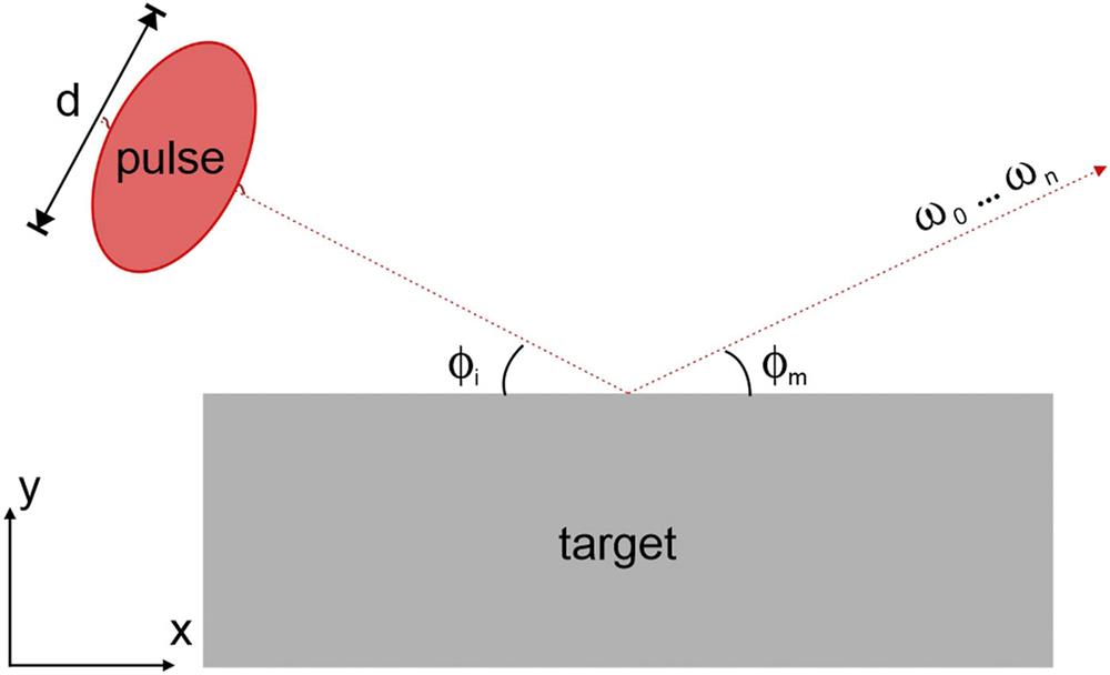
Fig. 1. Scheme of numerical simulation of HHG. d is the transverse dimension at full width at half maximum (FWHM), ϕ i is the angle of incidence, ϕ m is the angle of reflection, and ω 0, … , ω n are generated harmonics.

Fig. 2. (a) Typical electron density distribution in units of N cr, (b) field component E y in units of the relativistic electric field E rel, and (c) spatial spectrum of high harmonics in arbitrary units for 30 fs, focusing f /4, and a 0 = 30.
Fig. 3. (a) Typical spectrum of generated high harmonics in arbitrary units for the parameters of Fig. 2 and (b) typical time profile of electric field component after the interaction of the laser pulse with the target surface in units of E rel for 30 fs, focusing f /4, and a 0 = 30.
Fig. 4. Integral spectra of high harmonics at different laser pulse intensities. The colors show the spectra for different laser pulse intensities. The amplitude is in arbitrary units.
Fig. 5. Relative amplitude of harmonics [(a) and (c)] and averaged relative amplitude [(b) and (d)] as functions of incident laser pulse intensity (in W/cm2); different harmonics are shown by different colors. Dashed lines show approximation by a power function in (a) and (b) and approximation by a linear function in (c) and (d).
Fig. 6. Comparison of the integrated spectra of HHG at different angles of incidence of the laser pulse on the target for 30 fs, focusing f /4, and a 0 = 30. Spectra at different angles of incidence are shown by color. The amplitude is in arbitrary units.
Fig. 7. (a) and (c) Amplitudes of low (a) and high (c) harmonics as functions of focusing depth D for 30 fs, focusing f /4, and a 0 = 30; the amplitudes of different harmonics are shown by different colors. (b) and (d) Averaged relative amplitudes of harmonics as functions of focusing depth, taking into account low harmonics (b) and only high harmonics (d).
Fig. 8. Comparison of integrated spectra with and without density gradient for 30 fs, focusing f /4, and a 0 = 30. Spectra are shown in color for different density gradients. The amplitude is in arbitrary units.
Fig. 9. Density distribution at the moment of interaction of the laser pulse center with the target in the case of a sharp boundary (a) and in the case of a linear growth with L = 0.5λ 0 (b) for 30 fs, focusing f /4, and a 0 = 30. The density is normalized to N cr.
Fig. 10. (a) Amplitude of high harmonics as a function of density gradient scale for 30 fs, focusing f /4, and a 0 = 30; the amplitudes of different harmonics are shown by different colors. (b) Averaged relative amplitude of harmonics as a function of density gradient scale.


Set citation alerts for the article
Please enter your email address

© Copyright 2018-2021 | Chinese Laser Press. All Rights Reserved 沪ICP备15018463号-20