Weighted Sparse Cauchy Nonnegative Matrix Factorization Hyperspectral Unmixing Based on Spatial-Spectral Constraints

Shanxue Chen; Zhiyuan Hu

doi:10.3788/LOP213319

Journals >Laser & Optoelectronics Progress >Volume 60 >Issue 10 >Page 1028006 > Article

Laser & Optoelectronics Progress
Vol. 60, Issue 10, 1028006 (2023)

Weighted Sparse Cauchy Nonnegative Matrix Factorization Hyperspectral Unmixing Based on Spatial-Spectral Constraints

Shanxue Chen^1,2 and Zhiyuan Hu^1,3,*

Author Affiliations

¹Chongqing University of Posts and Telecommunications, School of Communication and Information Engineering, Chongqing, 400065, China

²Engineering Research Center of Mobile Communications of the Ministry of Education, Chongqing, 400065, China

³Chongqing Key Laboratory of Mobile Communications Technology, Chongqing, 400065, China

show less

DOI: 10.3788/LOP213319 Cite this Article Set citation alerts

Shanxue Chen, Zhiyuan Hu. Weighted Sparse Cauchy Nonnegative Matrix Factorization Hyperspectral Unmixing Based on Spatial-Spectral Constraints[J]. Laser & Optoelectronics Progress, 2023, 60(10): 1028006 Copy Citation Text

show less

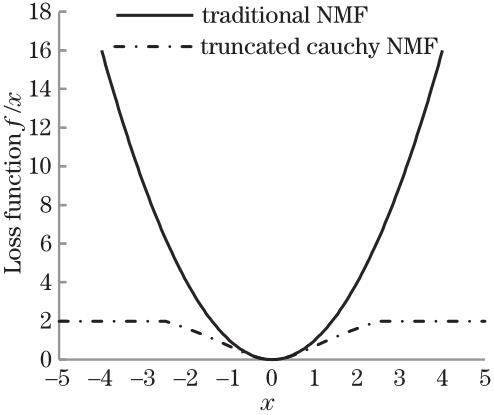
Fig. 1. Comparison of different loss functions

Download full size

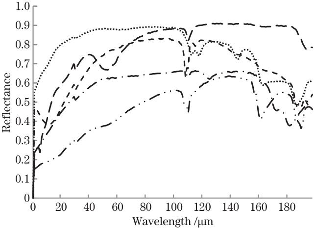
Fig. 2. Spectra of five ground objects in simulated data set

Download full size

Fig. 3. Average SAD and RMSE on Jasper Ridge data set for different

α

and

β

Download full size

Fig. 4. Comparison of SSCNMF algorithm for extracting endmembers on Jasper Ridge data set with real endmembers

Download full size

Fig. 5. Comparison of abundance maps on Jasper Ridge data set with real abundance maps by different algorithms

Download full size

Fig. 6. Comparison of SSCNMF algorithm for extracting endmembers on Urban data set with real endmembers

Download full size

Fig. 7. Comparison of abundance maps on Urban data set with real abundance maps by different algorithms

Download full size

Input：hyperspectral image matrix $R$ ，parameters $δ$ ， $α$ ，and $β$ ；

Initialization：initialize end element matrix $W^{0}$ and abundance matrix $H^{0}$ using VCA-FCLS；

Step1：calculate error matrix $E^{t} = \frac{R - W^{t} H^{t}}{γ_{t}}$ ；

Step2：calculate auxiliary matrix $X_{i j}^{t} = \frac{1}{1 + {(E_{i j}^{t})}^{2}}$ ；

Step3：calculate $e^{t} = \frac{1}{L * N} \sum R_{i j}$ ；

Step4：calculate $γ_{t + 1} = γ_{t} * \sqrt[]{\frac{1}{e^{0} - 1}}$ ；

Step5： $X^{t}$ cancel outliers to $X^{t + 1}$ ；

Step6：applying ASC constraints $R_{f} = [\begin{matrix} R \\ δ 1_{n}^{T} \end{matrix}]$ ， $W_{f} = [\begin{matrix} W \\ δ 1_{n}^{T} \end{matrix}]$ ， $X_{f} = [\begin{matrix} X \\ δ 1_{n}^{T} \end{matrix}]$ ；

Step7：update abundance matrix $H_{k j}^{t + 1}$ according to Eq.（20）；

Step8：update error matrix $E^{t + 1} = \frac{R - W^{t} H^{t + 1}}{γ^{t}}$ ；

Step9：update auxiliary matrix $X_{i j}^{t + 1} = \frac{1}{1 + {(E_{i j}^{t + 1})}^{2}}$ ；

Step10：update element matrix $W_{i k}^{t + 1}$ according to Eq.（22）；

Repeat above steps until stop condition is met；

Output：element matrix $W$ and abundance matrix $H$ .

Table 1. SSCNMF algorithm process

SNR /dB	MVCNMF	L_1/2-NMF	Cauchy NMF	SSRNMF	SSWNMF	SSCNMF
10	0.2573	0.2674	0.2466	0.2213	0.2160	0.2042
15	0.2041	0.1901	0.1843	0.1594	0.1565	0.1505
20	0.1655	0.1518	0.1511	0.0913	0.0944	0.0889
25	0.1098	0.0942	0.1035	0.0811	0.0735	0.0679
30	0.0917	0.0886	0.0872	0.0641	0.0537	0.0503

Table 2. SAD values after adding different levels of Gaussian white noise to each algorithm

SNR /dB	MVCNMF	L_1/2-NMF	Cauchy NMF	SSRNMF	SSWNMF	SSCNMF
10	0.4274	0.4118	0.4208	0.3473	0.3358	0.3069
15	0.3781	0.3710	0.3543	0.2873	0.2569	0.2381
20	0.2718	0.2556	0.2371	0.1519	0.1501	0.1477
25	0.1405	0.1289	0.1421	0.1088	0.0912	0.0784
30	0.1175	0.1052	0.1056	0.0733	0.0698	0.0595

Table 3. RMSE values after adding different levels of Gaussian white noise to each algorithm

D	MVCNMF	L_1/2-NMF	Cauchy NMF	SSRNMF	SSWNMF	SSCNMF
0.1	0.1565	0.1497	0.0831	0.0990	0.1074	0.0579
0.2	0.1996	0.1755	0.1463	0.1529	0.1406	0.0892
0.3	0.2136	0.2438	0.1986	0.1820	0.1885	0.1002
0.4	0.3853	0.3313	0.2965	0.2999	0.2734	0.1282

Table 4. SAD values after adding salt and pepper noise of different densities to each algorithm

D	MVCNMF	L_1/2-NMF	Cauchy NMF	SSRNMF	SSWNMF	SSCNMF
0.1	0.1281	0.1209	0.1093	0.0891	0.0857	0.0567
0.2	0.1687	0.1524	0.1678	0.1356	0.1426	0.0722
0.3	0.2349	0.2388	0.2116	0.1982	0.2031	0.1274
0.4	0.2968	0.2784	0.2849	0.2523	0.2382	0.1519

Table 5. RMSE values after adding salt and pepper noise of different densities to each algorithm

Category	MVCNMF	L_1/2-NMF	Cauchy NMF	SSRNMF	SSWNMF	SSCNMF
Tree	0.1474	0.1316	0.0913	0.1270	0.1112	0.1078
Water	0.1168	0.1239	0.1279	0.0792	0.0875	0.0558
Soil	0.0889	0.1179	0.1028	0.1457	0.0845	0.1203
Road	0.1358	0.1146	0.1256	0.1231	0.0981	0.0886
Mean	0.1224	0.1220	0.1119	0.1187	0.0953	0.0931

Table 6. SAD values of different algorithms on Jasper Ridge data set

Category	MVCNMF	L_1/2-NMF	Cauchy NMF	SSRNMF	SSWNMF	SSCNMF
Mean	0.2223	0.2011	0.2022	0.1871	0.1431	0.1367

Table 7. RMSE values of different algorithms on Jasper Ridge data set

Category	MVCNMF	L_1/2-NMF	Cauchy NMF	SSRNMF	SSWNMF	SSCNMF
Asphalt	0.2445	0.3580	0.2267	0.2772	0.2310	0.1806
Glass	0.3683	0.3324	0.2863	0.2118	0.2027	0.2015
Tree	0.2874	0.1935	0.3473	0.1347	0.1965	0.2204
Roof	0.1904	0.1471	0.2481	0.1923	0.1618	0.1647
Mean	0.2727	0.2578	0.2771	0.2040	0.1980	0.1918