Fig. 1. Ptychography. (a) Schematic of ptychography; (b) three sub-diffraction spots on Fraunhofer diffraction plane when an ideally spherical illumination is adopted; (c) three sub-diffraction spots when a non-spherical illumination is adopted

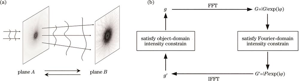
Fig. 2. G-S algorithm. (a) Schematic of G-S algorithm; (b) flowchart of G-S algorithm

Fig. 3. Optical path diagram and reconstruction results of radial translation multiple diffraction patterns phase reconstruction technology. (a) Schematic of radial multi-intensity CDI with ER algorithm; (b) one of recorded diffraction patterns; (c) modulus and phase of original object; (d) reconstructed object; (e) changes in reconstruction error with number of iterations for different overlap ratios

Fig. 4. Schematic of PIE

Fig. 5. Flowchart of annealing position-correcting algorithm^[22]

Fig. 6. Self-positioned scanning illumination optical path and reconstruction results^[52]. (a) Schematic of self-positioned scanning illumination method; (b) (c) amplitude and phase of reconstruction specimen

Fig. 7. Schematic diagram of divergent electron beam illuminating crystal^[54].(a) Change in illumination angle before and after shifting of probe; (b) kinematical diffraction of electron beam

Fig. 8. Reconstructed phase with different probe mode^[71]. (a) Static sample with single probe mode; (b) vibrating sample using square wave with single probe mode; (c) vibrating sample using sine wave with single probe mode; (d) static sample with five probe modes; (e) vibrating sample using square wave with five probe modes; (f) vibrating sample using sine wave with five probe modes

Fig. 9. Optical path and reconstruction results of single-shot PIE multi-beam illumination based on grating^[74]. (a) Setup of grating-based single shot PIE; (b) recorded diffraction-pattern array of a bee wing; (c) amplitude of reconstruction specimen; (d) phase of reconstruction specimen

Fig. 10. Optical path and reconstruction results of single-shot PIE multi-beam illumination based on pinhole array^[75]. (a) Single shot PIE setup with pinhole array; (b) reconstructed amplitude (top left) and phase (top right) of object, and reconstructed amplitude (bottom left) of probe, object measured by conventional microscope with 10× magnification(bottom right)

Fig. 11. CMI^[78]. (a) Schematic of CMI method; (b) recorded diffraction pattern; (c) amplitude on the entrance plane, dashed square shows support constraint; (d) amplitude of sample exit wave; (e) phase of sample exit wave

Fig. 12. Reconstructed results using $I^{n/\mathrm{2}}$ as Fourier-domain intensity constraint^[85]. (a)-(c) phase; (d)-(f) amplitude, where (a)-(f) correspond to n=1, 2, 3 respectively

Fig. 13. SR-PIE^[86]. (a) Flowchart of SR-PIE algorithm; (b) analysis of high spatial frequency contents reconstructed by SR-PIE, in which the left figure is the recorded diffraction spot, the data in the square area is used for light field reconstruction, the middle figure is the result of SR-PIE reconstruction, the distribution outside the box can correspond to the actual record, and the right figure is the error corresponding to each pixel; (c) left and right figures show the amplitude distribution reconstructed by PIE and SP-PIE respectively

Fig. 14. Principle and results of partial saturated diffraction reconstruction^[87]. (a) Convolution operation between G(u,v) and P(u,v); (b) resulting diffraction pattern E(u,v), the gray corresponds to saturation area and its width is smaller than 2W; (c) reconstructed USAF1951 target using datasets with varying degrees of saturation (bottom row), top row recorded diffraction patterns, inset is close-up of group 6 in USAF1951 target

Fig. 15. Typical applications of SXDM. (a) Ptychography image of freeze-dried D. radiodurans cells (right), top left is differential phase contrast image, bottom left is dark-field contrast image^[19]; (b) ptychography image of fossil diatom sample in water window (left), detailed view of the amplitude (top right) and phase (bottom right) corresponding to the marked area in left subfigure^[96]

Fig. 16. PXCT^[56]. (a) Experiment setup of PXCT; (b) reconstructed projection images from ptychographic data, left is amplitude, right is phase; (c) 3D rendering of tomographic reconstruction of bone sample, C and L represent osteocyte lacuna and connecting canaliculi, respectively

Fig. 17. Validity of SXDM with spectroscopy. (a) Reconstructed amplitudes and unwrapped phases of a mixture of PMMA and SiO₂ from five ptychographic data sets recorded at different energies, two curves are respectively experimental absorption spectra and calculated phase shift of PMMA^[112]; (b) X-ray microscopy of partially delithiated LiFePO₄, top is optical density maps from STXM (left) and ptychography (right) at 710 eV, bottom left is phase distribution from ptychography at 709.2 eV, bottom right is composition map^[113]

Fig. 18. Application of SXDM in wave diagnostics^[118]. (a) Reconstructed wave field in focus,amplitude encoded by brightness and the phase by color code; (b) scaled amplitude to highlight weak sidelobes; (c) horizontal slice of wave field along beam direction

Fig. 19. Wavefront distortion correction principle and results^[48]. (a) Retrieved wavefront deformation at exit plane of lens after subtracting an ideal spherical wave; (b) model of SiO₂ phase plate used to correct phase distortion; (c) contrast between beam caustics with and without phase plate, insets are respectively Ronchigram at the dotted position and logarithmic intensity distribution on focal plane

Fig. 20. Optical path and reconstruction results of beam splitting coding method^[186]. (a) Schematic of coded splitting imaging method; (b) phase distribution of designed pure-phase CSP, inset in top right shows close-up of region in red square; (c) reconstructed amplitude (left) and phase (right) of bee wings

Fig. 20. Ptychography electron microscopy imaging based STEM ^[135]. (a) Schematic of ptychographic electron microscopy using high-angle scattering, probe was scanned across the specimen using the microscope scanning coils; (b) diffraction pattern, central spot is bright-field intensity; (c) same diffraction pattern as (b) plotted on a log-intensity scale; (d) ptychographic reconstruction of gold particles

Fig. 21. Selected area ptychography principle and reconstruction results^[139]. (a) Schematic of selected area ptychography; (b) wrapped phase image, scale bar 100 nm; (c) contour plot of marked yellow area in Fig.21(b), contours have a spacing of 2π/100 rad

Fig. 22. Multimodal PIE technology^[141]. (a) Modes and effective sources of four sets of different partially coherent wave fields, in any set of data, these modes are orthogonal to each other and the numbers above them represent their contribution percentage; (b) specimen phase reconstructed with 16 modes; (c) reconstructed phase with a single mode

Fig. 23. Schematic diagram and reconstruction results of electronic Ptychography and 3PIE measurement of 3D structure^[142]. (a) Schematic of 3D ptychographic electron imaging, grayscale image in top right is TEM image of CNTs and red box indicates region where the ptychographic data recorded; (b) reconstructed phases at six positions along optical axis

Fig. 24. Schematic diagram of CMI based diagnostic setup in high power laser system^[156]

Fig. 25. Wavefront measurement results of high power laser system^[156]. (a) Recorded diffraction pattern, inset provides more details; (b) retrieved incident wave on plane of phase plate, left amplitude, right phase; (c) calculated intensity distributions near focal plane, distances between all adjacent planes are 4 mm; (d) obtained 3D focus intensity distribution; (e) reconstructed near-field amplitude after placing a USAF1951 target in front of focus lens

Fig. 26. Thermal distortions of high-repetition-rate laser amplifier measured with CMI method^[157]. (a) 1 Hz; (b) 5 Hz; (c) 7 Hz

Fig. 27. Schematic of measuring transmittance of optics based on PIE^[161]

Fig. 28. Measurement results of CPP^[49]. (a) Photograph of CPP with 310 mm diameter; (b) CPP design value; (c) measurement result of ZYGO interferometer; (d) wrapped phase distributions of CPP measured by ePIE; (e) unwrapped phase distributions of CPP measured by ePIE; (f) comparison of design value and ePIE measurement result along midperpendicular

Fig. 29. FPM^[170]. (a) FPM setup; (b) one of recorded low-resolution intensity images from a 2× objective lens in FPM; (c) reconstructed high-resolution phase image; (d) digital holography result with a 40× objective lens

Fig. 30. Reconstructed full FOV high-resolution image of blood smear (middle), insets show sample images and pupil functions (or aberrations) of five regions^[176]

Fig. 31. Single-shot FPM optical path diagram and reconstruction results ^[185]. (a) Setup of grating-based single-shot FPM; (b) recorded image array shown in log scale (left), normalized (0, 0) order subimage (right); (c) reconstructed amplitude (left) and phase (right) of bee wing

Fig. 33. Reconstruction analysis using PCGPA and ptychography algorithms^[191]. (a) Reconstruction error δ using PCGPA and ptychographic algorithm; (b) reconstructed pulses by PCGPA and ptychographic algorithm, signal-to-noise ratio is 8 dB, 20 dB, and 40 dB respectively; (c)(d) examples of pulse reconstruction from incomplete spectrograms using ptychographic algorithm, first plot is incomplete FROG trace for reconstruction, second plot is reconstructed trace, third plots and fourth plot are amplitude and phase of reconstructed pulses, fifth plot is changes in error δ with η, η is ratio of the number of pixels in incomplete trace used for reconstruction to the number of pixels in complete trace