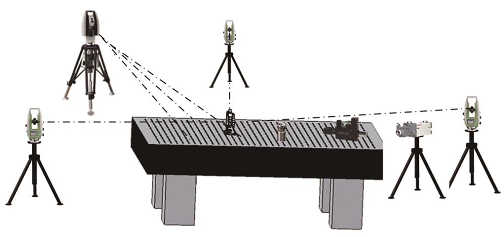
Fig. 1. Diagram of initial installation and adjustment

Fig. 2. Flowchart of model construction

Fig. 3. Structure diagram of shallow MLP and KAN. (a) Shallow structure of MLP; (b) shallow structure of KAN

Fig. 4. Structure diagram of KAN-Transformer

Fig. 5. Optical path diagram of a certain off-axis three-mirror optical system

Fig. 6. Production process of dataset

Fig. 7. MSE and MAE of different network structures under training dataset. (a) MSE; (b) MAE

Fig. 8. Linear distribution diagrams of small-scale predicted values and preset values based on Transformer. (a) X-decenter predicted values and preset values; (b) Y-decenter predicted values and preset values; (c) Z-decenter predicted values and preset values; (d) X-tilt predicted values and preset values; (e) Y-tilt predicted values and preset values; (f) Z-tilt predicted values and preset values

Fig. 9. Linear distribution diagram of small-scale predicted values and preset values based on KAN-Transformer. (a) X-decenter predicted values and preset values; (b) Y-decenter predicted values and preset values; (c) Z-decenter predicted values and preset values; (d) X-tilt predicted values and preset values; (e) Y-tilt predicted values and preset values; (f) Z-tilt predicted values and preset values

Fig. 10. Design residual wavefront aberration for F(0°, 0°), F(2°, -2°), and F(2°, 2°) fields of view. (a) F(0°, 0°); (b) F(2°, -2°); (c) F(2°, 2°)

Fig. 11. Simulating wavefront aberration in the fields of F(0°, 0°), F(2°, -2°), and F(2°, 2°) after misalignment. (a) F(0°, 0°); (b) F(2°, -2°); (c) F(2°, 2°)

Fig. 12. Wavefront aberration in the fields of F(0°, 0°), F(2°, -2°), and F(2°, 2°) after Simulated assembly. (a) F(0°, 0°); (b) F(2°, -2°); (c) F(2°, 2°)

Fig. 13. Prediction errors of different network structures

Fig. 14. Field of F(0°, 0°), F(0°, 2°), and F(2°, 2°) of PV error value and RMS error value of the system. (a) F(0°, 0°) PV error; (b) F(0°,2°) PV error; (c) F(2°, 2°) PV error; (d) F(0°, 0°) RMS error; (e) F(0°, 2°) RMS error; (f) F(2°, 2°) RMS error

Fig. 15. Training process of neural network with added noise

Table 1. Design parameters of three-mirror optical system

Table 2. Comparison between sensitivity matrix method calculation results and preset values

Table 3. Comparison between neural network calculation results and preset values

Table 4. Comparison between the second round sensitivity matrix method calculation results and preset values

Table 5. Comparison between the results of the second round of neural network calculations and the preset values

Table 6. Comparison between simulated noise training neural network of the first round of calculation results and preset values

Table 7. Comparison between simulated noise training neural network of the second round of calculation results and preset values