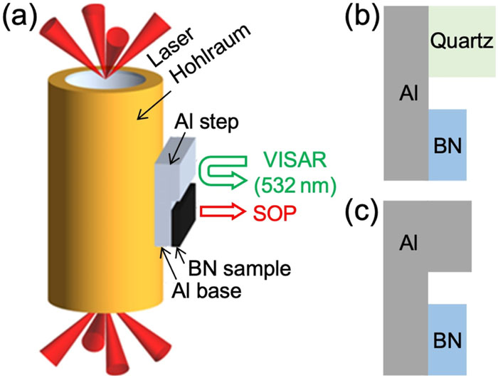
Fig. 1. (a) Schematic of experimental configuration. The planar sample package is attached to the side of the hohlraum. Two types of sample packages were used. (b) The first type consists of an Al pusher plate, the BN sample, and the quartz standard to measure the in situ shock velocity profile. (c) The second type uses an Al step instead of the quartz standard.

Fig. 2. Experimental configurations and typical data from the shots. The surface reflection and thermal emission signals were recorded by VISAR and SOP, for the Al base, BN sample, and quartz/Al-step standards. (a) Schematic of Al–BN–quartz-type EoS target. (b) Time-resolved VISAR and (c) SOP data for shot 043 using this type of target. t₁ marks the time when the shock crosses the interface between Al and BN, and t₂ marks the shock breakout time from the rear surface of the BN sample. After t₁, the shock propagates in the transparent quartz standard, with its shock front being monitored by VISAR. (d) Schematic of the Al–BN–Al-type target. (e) VISAR and (f) SOP data for shot 047. Three times are measured: t₁ is the time when the shock enters the BN sample, and t₂ and t₃ are the shock breakout times from the BN sample and the Al step, respectively. Since the our BN sample is porous, gradually increasing thermal emission ahead of shock breakout can be observed for BN, as shown in (c) and (f).

Fig. 3. Theoretical calculations of BN EoS at high pressures using the DFT-MD method, compared with previous results. (a) Principal Hugoniot calculated with three different choices of initial energy density E₀ with initial density 2.08 g/cm³. The Hugoniot with E₀ = −38.44 Ry/formula-unit best matches the previous experimental results (empty circles). (b) BN phase diagram in the pressure range relevant to this study. The best-match Hugoniot crosses the solid–liquid boundary at ∼1 Mbar pressure. The melting curve for c-BN (solid red) agrees well with the previous theoretical result (dashed green).

Fig. 4. Analysis of VISAR and SOP data for the Al–BN–quartz target in shot 043. The upper panel shows time-resolved SOP counts in the Al base, BN sample, and quartz standard. t₁ and t₂ are the shock breakout times from the rear surface of the Al base and BN sample, respectively. t₁ was determined as the half-height time of the rising edge of the SOP signals, while t₂ was determined as the half-height time of the corresponding dropping edge. The shock transit time through the BN sample is Δt_BN = t₂ − t₁. The lower panel shows the shock velocity profiles in the quartz standard, extracted from the two VISAR legs. The average quartz shock velocity calculated between t₁ and t₂ is used in the IM analysis.

Fig. 5. IM analysis in the pressure vs particle velocity plane for a typical shot using the Al–BN–quartz target (shot 046). The state of the quartz in this shot is determined by the intersection of the Hugoniot curve with the measured quartz Rayleigh line [plot (1)]. The Al release line going through this point is then determined. The intersections with the standard Al Hugoniot and the measured BN Rayleigh line determine the states of Al and BN along the respective Hugoniot [plot (2)]. Uncertainty ranges are shown by the dashed lines. The main source of errors in the IM analysis comes from the shock velocity measurements.

Fig. 6. Time-resolved X-ray radiation temperatures measured in the shots, illustrating the reproducibility of the X-ray drive. The unsteady-shock corrections calculated for the Al–BN–quartz shots 044 and 048 (solid lines) can be used in the Al–BN–Al shots 047 and 050 (dotted lines), respectively.

Fig. 7. Data analysis for the Al–BN–Al target in shot 047. The time-resolved VISAR and SOP counts in the Al base, BN, and Al are plotted. t₁, t₂, and t₃ are the shock breakout times from the Al base, the BN, and the Al step, respectively. These times were determined as the half-height positions of the corresponding rising/dropping slopes. The shock transit times in the BN and Al step were calculated as Δt_BN = t₂ − t₁ and Δt_Al = t₃ − t₁.

Fig. 8. Comparisons of theoretical BN Hugoniots with shock experiments. The data are presented in (a) the U_s–u_p plane and (b) the pressure–compression plane. For the theoretical curves, our DFT-MD Hugoniots for h-BN were calculated for the initial density 2.04 g/cm³ (solid black) and the initial density 2.08 g/cm³ (solid purple). The Hugoniot for c-BN (solid green) from Zhang et al.²³ was calculated starting from ρ₀ = 3.45 g/cm³ with model X2152. The experimental data for h-BN obtained in this study are shown in red. Our measurements and DFT-MD simulations are highly consistent up to 16 Mbar. As a comparison, the shock Hugoniot data for c-BN from previous experiments²³ and for h-BN from RUSBANK^15,16 are also shown.

Table 1. Shock Hugoniot data obtained from the Al–BN–quartz targets. $U_S^{\text{Q}}$ and $U_S^{\text{BN}}$ are the measured shock velocities of quartz and BN, respectively. The particle velocity $u_p^{\text{Al}}$ was calculated using the IM between the Al and quartz standards. The particle velocity $u_P^{\text{BN}}$, pressure P^BN, and compression ratio ${\rho }^{\text{BN}}/{\rho }_0^{BN}$ for shocked BN were determined by IM between the BN and Al. The uncertainties calculated by propagating the errors in the shock velocities are also shown.

Table 2. Shock Hugoniot data obtained from the Al–BN–Al target. $U_S^{\text{Al}}$ and $U_S^{\text{BN}}$ are the shock velocities measured in Al and BN. The particle velocity for Al, $u_p^{\text{Al}}$, was calculated from the Al Hugoniot. The particle velocity $u_P^{\text{BN}}$, pressure P^BN, and compression ratio ${\rho }^{\text{BN}}/{\rho }_0^{BN}$ for shocked BN were determined by IM between BN and Al. The uncertainties calculated by propagating the errors in the shock velocities are also shown.