Colored dissolved organic matter (CDOM) plays a pivotal role in the global carbon cycle and climate change. The rapid development of satellite remote sensing technology has provided a vast amount of ocean surface remote sensing data for oceanographic research, reflecting the internal state of the ocean to a certain extent. We combine multi-source ocean remote sensing data with deep learning techniques to propose a remote sensing inversion method for subsurface CDOM in the ocean. This method inverses the vertical distribution of subsurface CDOM by employing ocean surface remote sensing data, thus providing a new perspective and theoretical support for a deeper understanding of the mechanisms of the ocean carbon cycle and its interactions with climate change.

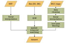
Firstly, the CDOM profile data obtained from BGC-Argo is preprocessed to address the uncertain vertical resolution. By conducting linear interpolation, the data is standardized to an interval of 1 m, ensuring consistency in depth between data points for subsequent analysis. Additionally, a low-pass filter is adopted to reduce peak fluctuations in the data, enhancing its smoothness and reliability. To address the missing ocean remote sensing data, we employ the inverse distance weighting (IDW) interpolation method, effectively filling in missing values in remote sensing images. The K-fold cross-validation method is utilized to evaluate the interpolation model, with the mean absolute percentage error (MAPE) selected as the evaluation metric. Given the spatial resolution mismatch between sea surface temperature (SST) data and remote sensing reflectance data, the bilinear interpolation algorithm is employed to reconstruct the resolution of the SST dataset, enhancing its resolution and ensuring spatio-temporal consistency of the model input data. Finally, based on the convolutional neural network (CNN) model, we design a subsurface CDOM inversion model for the ocean, adopting multi-band remote sensing reflectance, SST, and other parameters as inputs. This model consists of an input module, a CNN feature extraction module, and a prediction module, enabling the vertical distribution prediction of subsurface CDOM concentration in the ocean. As a result, the model’s applicability is evaluated via a test set and two independent test areas.

The filtered profile data of CDOM of the ocean exhibits smoother and more stable characteristics, effectively eliminating the interference of outliers on the overall data trend (Fig. 3). To achieve spatio-temporal consistency between BGC-Argo data and remote sensing reflectance data, we employ the IDW method to interpolate missing values in remote sensing reflectance images and validate the spatial interpolation model through K-fold cross-validation. By taking the Rrs443 remote sensing data from the first day of each month in 2020 as an example, the initial distribution of remote sensing data is shown in Fig. 4, while the reconstructed remote sensing data after IDW spatial interpolation is presented in Fig. 5. During cross-validation, the K value is set to 5, with the MAPE employed as the evaluation criterion. The results indicate that the overall error of the interpolation model remains below 30%, demonstrating the sound performance of the interpolation model. The proposed inversion model achieves a root mean square error (RMSE) of 0.14 μg/L, a correlation coefficient (r) of 0.73, and a coefficient of determination (R²) of 0.74 in the test set. Furthermore, in the validation of two independent test areas, the RMSE values are 0.13 μg/L and 0.18 μg/L respectively, with r values of 0.81 and 0.74, and R² values of 0.79 and 0.69 respectively. By analyzing the vertical distribution plots of predicted and actual values for independent test zones A and B (Figs. 8 and 9), combined with the residual scatter plot between predicted and actual values (Fig. 10), it is evident that the predicted values are mostly concentrated around the y=x diagonal with the actual values. This result demonstrates a high degree of consistency between the model’s predictions and the measured CDOM distribution characteristics, thereby confirming the validity and applicability of the proposed model. The correlation between the distribution of CDOM and SST is explored via the subsurface CDOM-SST scatter plot (Fig. 11), which further validates the rationality of the inversion results.

We leverage multi-band ocean remote sensing spectral data (B1: Rrs412; B2: Rrs443; B3: Rrs490; B4: Rrs510; B5: Rrs560; B6: Rrs665), SST remote sensing data, and BGC-Argo data, combined with a CNN model, to develop an inversion model for the vertical distribution of marine subsurface CDOM in the Northwest Pacific region (131°E?180°E, 26°N?54°N). To validate the accuracy of this model, we evaluate the performance of this model by adopting a test set, proving the model’s sound performance. Additionally, to further verify the model’s applicability, we conduct predictions for the vertical distribution of CDOM in two independent test areas, which reveals a high degree of consistency between the predicted and measured CDOM distribution characteristics, thereby proving the model’s effectiveness in presenting the vertical distribution characteristics of marine subsurface CDOM. Meanwhile, an analysis of the vertical distribution characteristics of subsurface CDOM in the Northwest Pacific region is conducted by utilizing the constructed vertical distribution maps of CDOM in the independent test areas. Notably, the mass concentrations in spring and summer are significantly higher than those in autumn and winter, with CDOM mass concentrations gradually increasing with depth. As a crucial component of the oceanic carbon cycle, the distribution and variation of CDOM significantly influence this cycle. We not only uncover these key features of the vertical distribution of marine subsurface CDOM but also provide a solid theoretical foundation and support for its inversion, facilitating a deeper understanding and prediction of the dynamic changes in the oceanic carbon cycle. However, our study has certain limitations. For instance, the IDW remote sensing data reconstruction method based on spatial correlation can be further optimized by incorporating factors such as time series to enhance the model’s ability to capture dynamic temporal changes. Additionally, considerations can be given to adjusting the model structure, increasing network depth, and exploring the inclusion of additional remote sensing parameters such as sea surface elevation and wind speed to delve deeper into the complex relationship between ocean remote sensing data and the vertical distribution of marine subsurface CDOM and improve prediction accuracy.

In 1996, McFeeters proposed the normalized difference water index (NDWI), leveraging the unique reflectance characteristics of water bodies in remote sensing images, high reflectance in the green band and low reflectance in the near-infrared band. This index enables effective extraction of water bodies from remote sensing images and has become a classic and widely cited method in water body extraction, with thousands of references in academic research. While NDWI is widely applied to remote sensing images, its application to airborne LiDAR point cloud data remains limited. Compared to remote sensing image data, airborne LiDAR offers advantages such as high-precision laser point cloud data acquisition, independence from solar radiation, and greater operational flexibility. To address this gap, we propose a novel NDWI-LiDAR method that facilitates the rapid and accurate extraction of water body information by using only the elevation data from dual-frequency laser point clouds, overcoming the dependence on full waveform data.

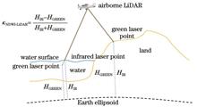
In this paper, the proposed NDWI-LiDAR leverages the uncertainty and measurement bias of green lasers in water surface measurements and is based on the point clouds generated by airborne infrared and green lasers. The expression form of this index is similar to that of the NDWI, but the pixel values of the near-infrared and green bands in remote sensing images are replaced by the elevations of infrared and green laser points. First, the raw measurement data from the infrared and green lasers are used to calculate the positions of the laser footprints, resulting in infrared and green laser point clouds, respectively. Second, the expression for NDWI-LiDAR is provided based on the different characteristics of infrared and green lasers in water and land measurements. Third, a land?water discriminator utilizing the NDWI-LiDAR is introduced, with the Otsu method applied to establish the threshold for water extraction. Finally, the pulse numbers of adjacent laser points are analyzed to differentiate and eliminate noisy water points, thus obtaining the final water surface laser points and realizing accurate water body extraction from airborne laser point clouds (Fig. 5).

The measurement datasets collected by the Optech CZMIL system are used to validate the correctness and effectiveness of the proposed method. In the experimental area, the NDWI-LiDAR values for land tend toward 0 and negative, whereas those for water are positive. As shown in the NDWI-LiDAR probability density distribution image (Fig. 10), the land and water NDWI-LiDAR data exhibit distinct dual peaks: the peak NDWI-LiDAR density value for water is approximately 0.3, whereas that for land is approximately 0. Compared with the traditional random sample consensus (RANSAC) method, which is based on single-frequency laser point clouds, the NDWI-LiDAR method proposed in this paper reduces the number of incorrectly extracted water points by 86.7% (Fig. 12). Equations (12) and (13) are used to calculate the distance bias and structural similarity (SSIM) index of the land?water interface determined by the two methods. The maximum bias, mean bias, and standard deviation of the land?water interface determined by the NDWI-LiDAR are 25.2, 4.2, and 4.2 m, respectively, with an SSIM value of 0.92. In contrast, the maximum bias, mean bias, and standard deviation determined via the RANSAC method are 50.3, 8.8, and 6.7 m, respectively, with an SSIM value of 0.89 (Table 1).

In the experimental area, the NDWI-LiDAR values for land tended toward 0 and negative values, whereas those for water are positive. From the perspective of the NDWI-LiDAR probability density distribution, the values for land and water significantly differ. The peak NDWI-LiDAR density for water is approximately 0.3, whereas that for land is approximately 0. The results indicate that the NDWI-LiDAR values for land and water are significantly different, suggesting that it is reasonable to use NDWI-LiDAR as a LiDAR-based index for water extraction. Compared with the traditional RANSAC method, which relies on single-frequency laser point clouds, the NDWI-LiDAR method proposed in this paper reduces the number of incorrectly extracted water points by 86.7%, reduces the standard deviation of the land?water interface by 37.3%, and improves the SSIM index by 3.3%. The results demonstrate that the NDWI-LiDAR method effectively leverages the advantages of dual-frequency laser point clouds, thus enabling accurate and efficient acquisition of spatial distribution information for water bodies based on LiDAR point clouds.