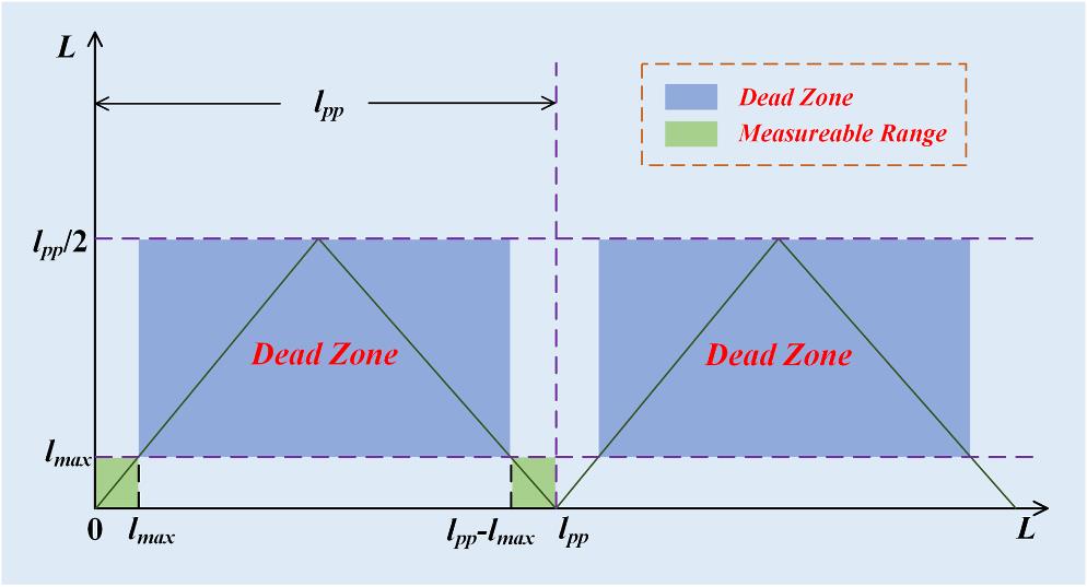
Fig. 1. Dead zones in the distance measurement when using chirped pulse interferometry. $l_{\mathrm{pp}}$ represents the pulse-to-pulse interval and is equal to $c/n_g\times f_{\mathrm{rep}}$. $c$ is the light speed in vacuum, $n_g$ is the group refractive index of air, and $f_{\mathrm{rep}}$ is the repetition frequency of the frequency comb. $l_{\max }$ is the measurable distance of chirped pulse interferometry, which is determined by the resolution of the OSA.

Fig. 2. Frequency comb interferometry in the frequency domain. (a), (b) In traditional spectral interferometry, the spectrum will be modulated and the modulation frequency is constant along the wavelength axis, e.g., the situations 2 and 3. Note that the spectrograms corresponding to the situations 2 and 3 are the same, despite that the distances are different. Limited by the resolution of the OSA, the spectrograms cannot be reconstructed when the distance is too large, e.g., the situation 4; (c), (d) Chirped pulse interferometry will occur when the reference pulses are chirped. The modulation frequency of the spectrograms is not constant, e.g., the situation 1, and there is a widest fringe. When the distances are changed, the position of the widest fringe changes, e.g., the situations 2 and 3. Note that the spectrograms corresponding to the situations 2 and 3 are not the same. Similarly, the spectrograms cannot be reconstructed when the distance is too large, e.g., the situation 4; (e), (f) The reference pulse is strongly chirped, and the pulse duration can well cover the pulse-to-pulse interval. The modulation frequency of the spectrograms is larger, and there is no dead zone along the measurement path.

Fig. 3. Recent progress in the field of distance measurement. Note that here we focus on the methods of spectral interferometry and chirped pulse interferometry. Some nice reviews can be seen in Refs. 67–69.

Fig. 4. Schematic of the measurement principle of the chirped pulse interferometry. H, hydrogen maser; MR, reference mirror; MM, measurement mirror; BS, beam splitter; OSA, optical spectrum analyzer. The local oscillator is greatly broadened by a highly dispersive fiber.

Fig. 5. Comparison between the spectral interferometry and the chirped pulse interferometry. (a) Spectrogram in the spectral interferometry with 0.4 mm distance. (b) Spectrogram in the spectral interferometry with 0.5 mm distance. We find that the fringe will be modulated when the distance is not zero, and the modulation frequency increases with increasing the distance. (c) Unwrapped phases for the 0.4 and 0.5 mm distances, respectively. The unwrapped phase increases linearly with increasing the optical frequency. (d) Phase difference between the phases in panel (c). The distance can be determined by the phase slope. (e) Spectrogram in the chirped pulse interferometry with 0.4 mm distance. (f) Spectrogram in the chirped pulse interferometry with 0.5 mm distance. We find that the modulation frequency of the fringe is no longer constant. The position of the widest fringe is shifted when changing the distance. (g) Unwrapped phases for the 0.4 and 0.5 mm distances, respectively. The unwrapped phase is not linearly but quadratically correlated with the optical frequency. (h) Phase difference between the phases in panel (g). We find that the phase difference is still linearly related to the optical frequency, and the distance can be also determined by the phase slope.

Fig. 6. Experimental results of real-time chirped pulse interferometry for absolute distance measurement. EDFA, Er-doped fiber amplifier; PD, photodetector; FS, fiber splitter; BS, beam splitter; C, collimator; M, mirror; CCR, corner reflector; HWP, half-wave plate; PBS, polarization beam splitter; QWP, quarter wave plate.

Fig. 7. (a) Measurement results using the OSA. (b) Measurement results using the oscilloscope.

Fig. 8. Relation between the time and the frequency. The pink solid circles show the raw data and the black line indicates the fitted curve. We find that time is linearly related to the frequency.

Fig. 9. Spectrograms corresponding to the different repetition frequencies. (a) Spectrogram when the repetition frequency is 250.0300035 MHz. (b) AC part of the spectrogram in panel (a). (c) Spectrogram when the repetition frequency is 249.99951875 MHz. (d) AC part of the spectrogram in panel (c). The position of the widest fringe is shifted to the right side (higher optical frequency) when the repetition frequency decreases slightly. This is because the pulse-to-pulse interval increases when decreasing the repetition frequency.

Fig. 10. Data process of the spectrograms in the frequency domain. (a) Wrapped phase of the spectrogram in Fig. 9(b). (b) Wrapped phase of the spectrogram in Fig. 9(d). (c) Unwrapped phases. The black solid line represents the unwrapped phase before changing the repetition frequency, and the red solid line shows the phase after changing the repetition frequency. The unwrapped phase is shifted to the right side. (d) Phase difference between the two phases in panel (c). We find a straight line whose slope can be used to determine the distances, despite that the unwrapped phase is not linearly related to the optical frequency.

Fig. 11. (a) Waveform with the target mirror at the initial position. (b) Waveform in one period of about 4 ns at the initial position. (c) AC part of the waveform in panel (b). (d) Waveform with the target mirror shifted by 100 mm. (e) Waveform in one period of about 4 ns after shifting the target mirror by 100 mm. (f) AC part of the waveform in panel (e). (g) Unwrapped phase of the waveform in panel (c). (h) Unwrapped phase of the waveform in panel (f). (i) Phase difference between the phases in panels (g) and (h), which is a straight line. (j) Wrapped phase of the signal in panel (c). (k) Wrapped phase of the signal in panel (f). Note that we change the horizontal axis to the wavelength, for the convenience of the phase measurements of the chosen wavelengths.

Fig. 12. Experimental results of the distance measurement. (a) Results of the coarse measurement with a 0.1-m step size in the 1 m range. The colorful solid points show the scatters of each measurement. (b) Results of the fine measurement with a 0.1-m step size in the 1 m range. The red x markers show the scatters of 1000 measurements. The black solid points indicate the average value, and the error bar shows twice the standard deviation. (c) Results of the coarse measurement with a 5-m step size in the 50 m range. The colorful solid points show the scatters of each measurement. (d) Results of the fine measurement with 5-m step size in the 50 m range. The red x markers show the scatters of 1000 measurements. The black solid points indicate the average value, and the error bar shows twice the standard deviation.

Fig. 13. Allan deviation at different averaging time.

Fig. 14. Experimental setup of ultrafast distance measurement. The target is a spinning disk with grooves of different depths.

Fig. 15. Experimental results of ultrafast distance measurement. The blue points represent the results using real-time chirped pulse interferometry, and the red points indicate the results measured by a coordinate measuring machine.

Fig. 16. Relation between the optical frequency and the time, taking into account the different orders of dispersion coefficients.

Table 1. Uncertainty budget of the absolute distance measurement.

Table 2. Coefficients of GVD at different orders.