 AI Video Guide
  AI Picture Guide
 AI One Sentence

Tobias Pahl, Felix Rosenthal, Johannes Breidenbach, Corvin Danzglock, Sebastian Hagemeier, Xin Xu, Marco Künne, Peter Lehmann, "Electromagnetic modeling of interference, confocal, and focus variation microscopy," Adv. Photon. Nexus 3, 016013 (2024)
- Advanced Photonics Nexus
- Vol. 3, Issue 1, 016013 (2024)
Note: This section is automatically generated by AI . The website and platform operators shall not be liable for any commercial or legal consequences arising from your use of AI generated content on this website. Please be aware of this.
Abstract
Keywords
1 Introduction
Optical surface topography measurement techniques, such as coherence scanning interferometry (CSI) being representative for interference microscopy, confocal microscopy (CM), and focus variation microscopy (FVM) are widespread for fast and contactless measurement of geometrical surface features, down to lateral dimensions of several 100 nm and an axial resolution down to the subnanometer range, depending on the respective measurement technique. All of the three named measurement methods show advantages compared to each other with respect to characteristics, such as axial resolution (CSI),1,2 lateral resolution (CM),3,4 or the capability of measuring steep slopes (FVM).5,6 A detailed description of common surface topography measurement instruments is out of the scope of this paper but is provided in a book edited by Leach.7 Further, it should be noted that besides surface topography inspection, measurement techniques as CSI or CM are also used in other fields of application, such as 3D imaging of biological samples. Several other familiar terms, such as white-light interferometry or optical coherence tomography, refer to CSI techniques.1,8 Depending on the field of application parameters, such as the illumination wavelength or numerical aperture (NA) as well as the signal processing algorithm, can differ, leading to different specifications of system characteristics, such as the lateral or axial resolution. In this study, we focus on surface topography measurement techniques operating with light in the visible range.
Due to the wave properties of light and resulting diffraction effects, optical profilers always suffer from systematic deviations occurring with respect to certain surface characteristics and system parameters.9
Generally, simulation models of optical surface profilers are either quasianalytic or rigorous models depending on the computation of the light scattering process. Usually, quasianalytic models require less computation time and memory. They also provide better physical insight in the imaging and scattering processes and are hence often preferred over rigorous models. On the other hand, rigorous simulations show higher accuracy, since no approximations are made. As the modeling of the measurement instruments is the main focus of this study, we concentrate on quasianalytic scattering theory. The scattering model, which describes the light–surface interaction, is usually independent of the instrument modeling and can therefore be changed if necessary. Further, surface textures typically measured by FVM may have geometrical dimensions that are too large to calculate scattered fields rigorously in reasonable time. Thus for rigorous modeling, we refer to previous publications for CSI21 and CM.22
Sign up for Advanced Photonics Nexus TOC. Get the latest issue of Advanced Photonics Nexus delivered right to you!Sign up now
In the previous studies, quasianalytic models are developed based on Fourier optics or scalar Kirchhoff theory to analyze systematic deviations and the transfer characteristics of CSI systems,15,23
It should be noted that with respect to the scattering surface, the so-called phase object approximation15,19,27 and foil model23,25,29 are based on the same scalar Kirchhoff scattering theory31 and thus show similar results.19,32 Generally, the phase object approximation is more flexible regarding incidence angle and surface material dependence of reflection coefficients and is less affected by numerical artifacts. As an additional advantage, the phase object approach can be simply exchanged by a rigorous method in the modeling of surface topography instruments if required, since both may be considered by a pupil integration. The foil model describes the surface as an infinitely thin foil-like object and considers the measurement process by a 3D convolution of the foil with the 3D point spread function (PSF) corresponding to the measurement instrument, which is calculated from the 3D transfer function (TF). Lehmann and Pahl30 presented an analytic calculation of the 3D TF for conventional microscopes and CSI33 enabling a fast computation of the 3D PSF. An extremely quick computation of CSI results is enabled by multiplying the 2D Fourier transform of the phase object with a cross section of the analytic 3D TF resulting in the scalar so-called universal Fourier optics (UFO) model.34 A comparison of the so-called elementary Fourier optics model,35 which is similar to the UFO model but approximates the cross section of the 3D TF by the conventional modulation transfer function, the UFO model, and the foil model is provided by Hooshmand et al.32
However, if imaging systems of high NA larger than 0.6 are applied, a vectorial treatment is appropriate, since polarization-dependent focusing and reflectivity become important, as mentioned by Totzeck.36 Further, dark-field illumination, which is usually applied in FVM, implies large angles of incidence as well and hence requires a vectorial treatment. Due to the trend toward miniaturization of surface features, demands on the resolution of optical profilers increase continuously. Therefore, systems of high NA or additional dark-field illumination are being developed, leading to increasing challenges in modeling.
Rahlves et al.14 presented a vectorial signal modeling of CM. However, lateral scanning, which is one major and time-consuming task in CM modeling, is not considered. Xie27 developed a scalar model based on the vector theory of Richards and Wolf37 describing the field in the focus of a microscope objective lens. Nonetheless, the model presented by Xie only considers the zeroth order of diffraction for depth scan, leading to significant disadvantages compared to the conventional Kirchhoff model as demonstrated in a previous study.19 A vectorial extension of the scalar Kirchhoff model for CSI has been presented by Pahl et al.19 However, the model shows inconsistencies, since the electric field is not perpendicular to the wave vector after the scattering process anymore. These inconsistencies are partially fixed in a recent publication.20 Here the remaining inconsistencies are fixed and not only CSI, but also CM and FVM, are modeled similarly. For validation, results obtained from the vectorial model are compared to measurement results for all three instruments.
2 Model of Optical Imaging Profilometry
Generally, simulation models of microscopic arrangements can be split into three parts, illumination, light–surface interaction, and imaging as described by Totzeck.36 Since the light–surface interaction and the microscopic imaging are similar for all three measurement techniques, we first focus on modeling the scattering and imaging process of plane waves scattered at the sample’s surface. Afterward, we present the modeling of illumination and other properties, which differ among the measurement techniques. Further, we restrict the modeling to surface profiles that are invariant under translation in one dimension (here
The models of the microscopic arrangements presented in this study are based on general integral formulations, which are numerically implemented by sums, and are used in the same way with rigorous scattering models. It should be noted that under certain circumstances faster implementations, such as the UFO model34 for CSI exist, where properties of the measurement instruments are considered by analytically calculated 3D TFs. However, these specifications are based on the same theory, require a deeper understanding of the imaging system, and are more complicated to implement, especially if angle or material-dependent properties need to be considered.
2.1 Scattering Theory
The scattering theory presented by Beckmann38 is a scalar theory based on the Kirchhoff approximation. However, in order to consider microscope objective lenses of high NA, a vectorial extension of the scattering model is required. Thus, we first present the scalar model and afterward show the vectorial extension.
2.1.1 Scalar model
In the scalar model, the electric object (o) field is restricted to a scalar field distribution
![]()
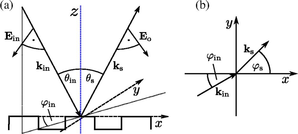
Figure 1.Sketch of the scattering geometry including definitions of wave vectors, electric fields, and angles of incidence in (a)
The general scattering theory derived by Beckmann38 describes the scattered field by an integration over the area
Assuming a periodic surface profile
2.1.2 Vectorial extension
If objective lenses of high NA or dark-field illumination are used, a vectorial treatment of the scattering process increases the accuracy of modeling. Hence, the scalar field distribution of Sec. 2.1.1 is extended to the vectorial electric field
In order to split the incident field into parallel and perpendicular parts, the unit vectors
The components of the electric field are then given by
In order to compute the incident electric field
It should be mentioned that the Kirchhoff theory is limited to surface profiles with radii of curvature, which are large compared to the wavelength of light,31,38,41 and effects such as multiple scattering, polarization-dependent diffraction, and shadowing are not considered. Further studies on the validity of the Kirchhoff approximation are given by Thorsos42 and Thorsos and Jackson.43 However, if the validity of the Kirchhoff approximation is not given, the Fourier coefficients [see Eq. (9)] can be calculated rigorously using FEM for scalar44 and vectorial21,22 coefficients, with the drawback of long computation time and large computer memory requirements. Therefore, the implementation is performed in a way that the scattered field computation method can be changed without changing the modeling of the imaging technique.
For 3D surface profiles, the Fourier series [Eq. (3) for scalar and Eq. (6) for vectorial] needs to be calculated depending on two spatial coordinates,
2.2 Microscope Models
The scattered electric field for plane wave illumination can be calculated according to Eq. (6) for all of the presented instruments. However, there are effects, such as coherence and interference, that need to be considered, depending on the measurement method. Note that aberrations, apodization, and inhomogeneous illumination can be simply considered by pupil functions as described in Refs. 21 and 22 but are neglected in this study for simplicity if not explicitly mentioned otherwise.
2.2.1 Coherence scanning interferometry
A schematic representation of a coherence scanning interferometer in Linnik configuration is shown in Fig. 2(a). Note that there are other frequently used CSI arrangements, such as Michelson or Mirau configurations, the modeling of which is similar. The illumination beam path sketched in the figure in red corresponds to Köhler illumination.3 Hence, a spatially extended light source represented by the diffuser is imaged in the back focal plane of the objective lenses leading to plane incident waves of certain angles of incidence with respect to the object and the reference mirror. Therefore, each plane wave incident under a certain angle originates from another point of the light source and, thus, the illumination is spatially incoherent. As a consequence, the intensity
![]()
Figure 2.Schematic representations of (a) a coherence scanning interferometer in Linnik configuration, (b) a confocal microscope with spinning disk for lateral scanning, and (c) a focus variation microscope with ring light illumination. The illumination beam path is sketched in red (bright-field), the imaging beam path in blue, and the dark-field ring light (RL) is shown in green in the case of FVM. D, diffuser; CL, condenser lens; RM, reference mirror; MO, microscope objective; BSC, beam splitter cube; TL, tube lens; C, camera; PS, piezo stage; S, sample; PHD, pinhole disk; and FL, field lens.
For a polychromatic light source with the spectrum
2.2.2 Confocal microscopy
A schematic representation of a confocal microscope is displayed in Fig. 2(b). Compared to CSI, a rotating pinhole disc is placed in the illumination as well as in the imaging beam path. The pinholes in the illumination path can be considered as single-point sources emitting spatially coherent light. Since only small spots on the object’s surface are illuminated by these pinholes, the pinhole disk rotates, leading to a lateral scanning of the measured surface section. The lateral scan can be considered in the simulation describing the field from a single pinhole, which is incident on the surface, in the pinhole plane by a
Considering infinitely small pinholes or a spatially coherently illuminated pinhole disk, we can set
2.2.3 Focus variation microscopy
A schematic of a focus variation microscope is shown in Fig. 2(c). Similar to CSI, the bright-field illumination corresponds to Köhler illumination. Therefore, the total intensity is given by integration over all intensities obtained for plane incident waves within the NA of the objective lens, as shown in Eq. (13). Since no reference mirror exists, the intensity
3 Results
To validate the simulation model, results are exemplarily compared to measurement results obtained by CSI, CM, and FVM. As an example, sinusoidal surface profiles fulfilling the validity conditions of the Kirchhoff approximation will be examined. On the one hand, measurements of sinusoidal surfaces may show systematic deviations;2,21 and on the other hand, the definition of the instrument transfer function (ITF), used for characterization of topography measurement instruments, is based on the measurement of sinusoidal surface topographies.35 Hence, a precise modeling of the topography measurement process of sinusoidal surfaces is of particular interest. For CSI and CM, a sinusoidal standard (Rubert 54345) with period length
It should be mentioned that simulations are validated by comparison with cross sections of 3D topography measurements in the
It should be mentioned that we focus on an exemplary comparison between simulation and measurement to demonstrate that typical effects in optical surface topography measurement are reliably reproduced by the presented simulation model. Since the modeling of four different measurement instruments already requires a lot of explanation, a more general comparison is outside the scope of the paper. In order to underline the requirement of vectorial modeling, a comparison between results simulated using the vectorial and the scalar approach is shown exemplarily for CM in Fig. 9 in the Appendix.
3.1 Coherence Scanning Interferometry
CSI results are obtained using a 50× Mirau interferometer of
A simulated image stack related to a single camera line is shown in Fig. 3(a); the corresponding measurement result is displayed in Fig. 3(b). Note that after offset subtraction, the intensities are normalized by the maximum intensity. The
![]()
Figure 3.(a), (c) Simulated and (b), (d) measured results for a sinusoidal surface profile of period length
Figures 3(a) and 3(b) show good agreement. Both patterns are sinusoidally modulated with respect to the lateral
Surfaces are reconstructed using conventional CSI signal processing algorithms.2,51 The result of the analysis of the envelope’s maximum position is named envelope profile, and the result obtained by phase analysis combined with fringe order detection using the envelope is referred to as phase profile. Reconstructed sinusoidal profiles obtained from simulation and measurement are presented in Figs. 3(c) and 3(d). In both figures, the reference profile, which is given by the nominal profile for simulation and by an AFM measurement result in the experimental case, is shown in black for comparison. The evaluation wavelength
The simulated as well as measured envelope profiles show an amplitude that is more than 3.5 times larger compared to the nominal PV amplitude of
Due to the overestimation of the envelope profile’s amplitude, the phase profiles suffer from phase jumps, which follow from an incorrect estimation of the fringe order through the envelope detection.2 In order to get rid of these phase jumps, an unwrapping procedure is applied, leading to the profiles shown in green. For measurement and simulation, the amplitudes of the unwrapped phase profiles are smaller compared to the nominal height, which is consistent with expectations derived from the 3D TF33 and from known ITFs35 defined in particular by the output amplitude of a measured sinusoidal profile normalized by the real amplitude.
In order to verify simulation results for microscope arrangements of high lateral resolution, Fig. 4 shows simulated [Figs. 4(a) and 4(c)] and measured [Figs. 4(b) and 4(d)] results of the same sinusoidal standard measured by a 100× Linnik interferometer as sketched in Fig. 2(a) of
![]()
Figure 4.(a), (c) Simulated and (b), (d) measured results from a sinusoidal surface profile of period length
As expected, due to the higher NA and the resulting smaller depth of field52 resulting in a limited longitudinal spatial coherence,50 the envelope in both simulated and measured interference signals [see Figs. 4(a) and 4(b)] is narrower compared to the envelopes for
In this context, it should be noted that setting up and adjusting a Linnik interferometer, especially of high NA, is much more challenging than building Mirau or Michelson interferometers. The Linnik configuration requires two objective lenses that are assumed to be identical but are not fulfilled in reality. In addition, both objectives have to be placed at the same distance from the beam splitter cube and adjusted with respect to the optical axis. Due to the high NA and the small depth of field, even small deviations from the ideal adjustment cause deviations in the measurement results. Therefore, deviations obtained between the simulated and measured results probably follow from slight, inevitable misalignment and objective or beam splitter mismatch, finally leading to deviations in measured results. Analyzing the influence of maladjustment and aberrations on simulated results is outside the scope of this study but can be principally included in the simulation model by appropriate pupil functions, as shown elsewhere.3,53,54
Figures 4(c) and 4(d) display envelope and phase (
Nonetheless, measurement results for both the Mirau and the Linnik interferometer are reliably reproduced by the simulation.
3.2 Confocal Microscopy
Results of a confocal microscope as sketched in Fig. 2(b) are simulated for a
Figure 5 shows CM results obtained again from the sinusoidal surface standard (Rubert 543) using a cyan light source of
![]()
Figure 5.(a) Simulated and (b) measured intensity responses obtained from a sinusoidal surface profile of period length
Figure 5 displays simulated [Fig. 5(a)] and measured [Fig. 5(b)] intensity signals depending on the lateral
For better comparability, cross sections at fixed
Profiles reconstructed by Gaussian approximation18 are displayed in Fig. 5(d). For reference, a profile measured by an AFM and the nominal surface profile are additionally shown. The PV amplitudes correspond to the nominal amplitude for both measured and simulated profiles. Due to the larger pixel width of the camera compared to the CSI setup, the surface’s microroughness is no longer present in the measured result.
In sum, measured and simulated intensities as well as evaluated profiles show good agreement.
3.3 Focus Variation Microscopy
FVM results are obtained for a 10× microscope objective lens of
Since the axial resolution of focus variation microscopes is in the range of micrometers, a Rubert 525 sinusoidal standard45 is examined. It should be noted that usually rough surfaces are required to achieve reliable FVM results. However, for comparison and validation of the simulation model, it is more reasonable to use a specular surface with deterministic texture. The influence of an additional microroughness superimposing the deterministic sinusoidal surface is demonstrated in simulation later in this section. Measurements and simulations are performed using only bright-field, only dark-field, and combined illumination to study the impact of both illumination types separately. The refractive index of nickel is assumed to be constantly
Figure 6 displays simulated [Figs. 6(a), 6(c), and 6(e)] and measured [Figs. 6(b), 6(d), and 6(f)] normalized intensities obtained by depth scans. Comparison between simulated and measured results shows good agreement for all three illumination configurations. In case of only bright-field illumination [Figs. 6(a) and 6(b)], bright spots from the peaks and valleys of the surface appear in the focus of the objective lens. Out of focus, the bright spots blur as expected. Almost no information is captured by the camera from the slopes of the surface due to the limited NA of the objective lens, which can be seen by the dark spots between the bright spots.
![]()
Figure 6.(a), (c), (e) Simulated and (b), (d), (f) measured normalized intensity depth responses obtained from a sinusoidal surface profile of period length
Compared to bright-field illumination, results obtained with dark-field illumination show maximum intensities at the slopes of the profile in focus. This observation meets the expectation, since specular reflection occurs at the peaks and valleys, and hence this light is not captured by the objective lens for dark-field illumination. Comparing simulated and measured results, the measured result shows an additional modulation occurring as three bright stripes in the intensity, as marked by the green arrows in Fig. 6(d). In contrast to the simulation, where the ring light is assumed to be homogeneous, in practice the ring light is implemented in three layers, as reported by Xu et al.,17 providing a simple explanation for the slight deviations between measurement and simulation.
Figures 6(e) and 6(f) present results obtained for a combination of bright- and dark-field illumination, where
Figures 7(a) and 7(b) display profiles obtained from the intensity signals shown in Figs. 6(e) and 6(f). The profile reconstruction is performed as described by Xu et al.17 using five pixels to calculate the standard deviation as a measure of contrast. For reference (marked as ref. in Fig. 7), the nominal profile is shown in Fig. 7(a). In Fig. 7(b), the reference profile is obtained by the tactile stylus instrument MarSurf GD26. The microroughness of the measured profile resulted in an arithmetic mean value
![]()
Figure 7.Surface profiles (eval.) obtained from (a) simulated and (b) measured depth response signals depicted in
Comparison of Figs. 7(a) and 7(b) shows good qualitative agreement. In both cases, the period length and the PV height can be extracted from the measured data with the accuracy provided by the method. However, the sinusoidal shape of the surface profile is reproduced neither by the measurement nor by the simulation. This significant deviation from the reference profile is caused by the fact that the surface shows a specular reflection, i.e., the microroughness superimposing the profile is very low. Therefore, the intensity obtained from the local areas of low surface slope is much greater compared to the intensity captured from light reflected at the sloped areas. Hence, the maximum contrast, which is related to the measured surface height as described by Xu et al.,17 is detected from out-of-focus light reflected from the areas of low surface slope instead of the in-focus light from the sloped areas [see Figs. 6(e) and 6(f)]. Slight deviations between measurement and simulation again follow from different types of dark-field ring light.
In order to demonstrate the influence of microroughness on the measurement accuracy, Figs. 7(c) and 7(d) show simulated intensity signals [Fig. 7(c)] and the corresponding profile reconstruction [Fig. 7(d)] obtained from the same sinusoidal surface profile, but with a superimposed microroughness contribution of
In summary, simulated and measured results are in good agreement for all three types of illumination. Although a specular sinusoidal surface profile is not an intended measurement object for FVM measurements, it validates the simulation model and so allows one to identify any maladjustment of the microscope setup. However, as is well known, higher microroughness is required for reliable reconstruction of the surface topography based on FVM.
4 Conclusion
An accurate, quasianalytic modeling of the three most widespread optical techniques for surface topography measurement is presented. In order to model instrumental configurations providing high lateral and axial resolution as well as enabling measurements of steeply sloped surfaces, the scalar Kirchhoff modeling of scattering is extended to a vectorial treatment. Therefore, several rotations of the electric field during the focusing and scattering processes are to be considered. Simulations are performed and validated by comparison with measurement results for
Measurements and simulations are obtained for sinusoidal surface profiles, as these profiles comply with the restrictions of the Kirchhoff approximation; they are often used for system characterization such as ITF estimation and can cause systematic deviations in measurement results due to the high-frequency components of sinusoidal phase gratings. For all of the studied measurement configurations, measured intensities as well as reconstructed profiles are reproduced accurately.
Since the modeling is based on analytic assumptions, simulation results are obtained in a timely fashion. However, for more complex surface profiles, which do not fulfill the requirements of the Kirchhoff approximation, the model is implemented in a way that Fourier coefficients can be calculated rigorously, while everything else remains unchanged.
In sum, an accurate model of most-used instruments for surface topography measurement is provided. The reliability of the modeling has been checked, especially with respect to measurement instruments of high lateral resolution for 2D surface profiles. However, an extension to 3D surfaces is straightforward. The model is simple, and fast, gives insight into physical mechanisms of imaging and scattering, and enables detailed studies of measurement performance for certain surface profiles and instrument configurations. Thus, the model can identify suitable measurement instruments and configuration for a certain application without great effort and cost.
In future studies, more quantitative comparisons, including an error estimation between simulated measured results, will be established. In addition, more detailed comparisons between scalar and vectorial models are of great interest, as most of the common simulation models are based on scalar theory. Moreover, the model can be used to investigate the limits, according to which surface topography measurement processes are subject to the linear transfer behavior of the instruments. In general, the model needs to be validated for more complex 2D and 3D surfaces by comparison to rigorously simulated as well as measured results. In addition to the rigorous models published by the authors (see Refs. 21 and 22), comparisons can be performed using more generally applicable commercial software, such as VirtualLab Fusion.56
5 Appendix
5.1 3D Surface Topographies
For clarity reasons, Figs. 3–5 display 2D profiles of 3D surface topographies measured with Mirau, Linnik, and confocal microscopes, respectively. Figure 8 shows 3D surface topography reconstructions for better credibility of the measurement results. The positions where the profiles are extracted are marked by black lines. Since the surface topography reconstruction of specular surfaces using FVM (Fig. 7) suffers from missing sloped areas, we refrain from showing the 3D surface topography here.
![]()
Figure 8.Extracts of measured surface topographies obtained by a (a) Mirau and (b) Linnik interferometer as well as a (c) confocal microscope. The sections, where the profiles shown in
5.2 Comparison of the Scalar and Vectorial Approach
Differences between the scalar approach (Sec. 2.1.1) and the vectorial extension (Sec. 2.1.2) are demonstrated in the example of a 100×
![]()
Figure 9.Results obtained from a sinusoidal surface profile of period length
Tobias Pahl received his master’s degree in physics in 2018 from the University of Münster. He has been working as a research assistant and a PhD candidate in the Measurement Technology Group of the Department of Electrical Engineering and Computer Science at the University of Kassel since 2019. His main research interests are interference, focus-variation, and confocal microscopes with high lateral resolution and their modeling.
Felix Rosenthal worked in the field of measurement technology at the University of Kassel, Germany, after completing his master’s degree in physics. He has been a research assistant since 2023 and is working on his dissertation. His research focuses on the determination of the 3D transfer function of optical instruments and the processing of data.
Johannes Breidenbach completed his bachelor’s degree in 2022. During his bachelor’s thesis and his work as a student research assistant, he mainly dealt with the vectorial electromagnetic modeling of coherence scanning interferometry.
Corvin Danzglock received his master’s degree in electrical engineering in 2023. His master’s thesis dealt with efficient modeling of focus-variation microscopes. Since 2023, he works as a software engineer in an industrial company.
Sebastian Hagemeier has been working as a research assistant in the Department of Metrology at the University of Kassel, Germany, since October 2014. He completed his doctorate degree in engineering sciences in February 2022. His scientific work includes the comparison of the transfer behavior of various surface topography sensors in a multisensor measuring system. He is also working on the development and investigation of a fiber-coupled confocal-interferometric distance sensor for precise high-speed profilometry.
Xin Xu is a research employee in the Department of Messtechnik at the University of Kassel, Germany, since October 2019 and she did her doctorate meanwhile. She studied sensor system technology at the University of Applied Science, Germany and electrical communication engineering at the University of Kassel, Germany. She worked at an international company named USTER in China as a sensor engineer.
Marco Künne completed his master’s degree in nanoscience in 2019. Since then, he has been working on his PhD at the University of Kassel in the field of optical metrology, specifically focusing on high-resolution Linnik interferometry. His academic research includes the development of precise optical setups as well as data processing and the work on new techniques for data evaluation.
Peter Lehmann studied physics at the University of Karlsruhe, Germany. He received his PhD in engineering at the University of Bremen in 1994 and received his habilitation degree in 2002. From 2001 to 2008, he coordinated research projects related to optical metrology in an industrial company. Since 2008, he has been a full professor and holds the chair in measurement technology at the Faculty of Electrical Engineering and Computer Science, University of Kassel, Germany.
References
[1] P. de Groot, R. Leach. Coherence scanning interferometry. Optical Measurement of Surface Topography, 187-208(2011).
[3] T. R. Corle, G. S. Kino. Confocal Scanning Optical Microscopy and Related Imaging Systems(1996).
[4] R. Artigas, R. Leach. Imaging confocal microscopy. Optical Measurement of Surface Topography, 237-286(2011).
[7] R. Leach. Optical Measurement of Surface Topography(2011).
[8] D. Malacara, J. Schmit, K. Creath, J. Wyant. Surface profilers, multiple wavelength, and white light interferometry. Optical Shop Testing, 667-755(2007).
[18] S. Hagemeier. Comparison and investigation of various topography sensors using a multisensor measuring system(2022).
[27] W. Xie. Transfer characteristics of white light interferometers and confocal microscopes(2017).
[38] P. Beckmann, A. Spizzichino. The Scattering of Electromagnetic Waves from Rough Surfaces(1987).
[39] W. Singer, M. Totzeck, H. Gross. Handbook of Optical Systems. Volume 2: Physical Image Formation(2006).
[40] J. A. Ogilvy, H. M. Merklinger. Theory of Wave Scattering from Random Rough Surfaces(1991).
[41] J. Ogilvy. Wave scattering from rough surfaces. Rep. Progr. Phys., 50, 1553(1987).
[45] Rubert & Co Ltd., (accessed 30 January 2023).
[46] Cantilever Tap190Al-G(2023).
[51] S. Tereschenko. Digitale Analyse periodischer und transienter Messsignale anhand von Beispielen aus der optischen Präzisionsmesstechnik(2018).
[52] R. Leach, R. Leach. Some common terms and definitions. Optical Measurement of Surface Topography, 15-22(2011).
[53] R. Shannon, J. Wyant, K. Creath, J. Wyant. Basic wavefront aberration theory for optical metrology. Applied Optics and Optical Engineering, 1-54(1992).
[55] Geometrical product specification (GPS)—surface texture: profile method—terms, definitions and surface texture parameters(2010).


Set citation alerts for the article
Please enter your email address

© Copyright 2018-2021 | Chinese Laser Press. All Rights Reserved 沪ICP备15018463号-20