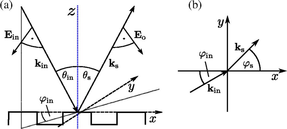
Fig. 1. Sketch of the scattering geometry including definitions of wave vectors, electric fields, and angles of incidence in (a) $x\text{–}z$ plane and (b) $x\text{–}y$ plane. The optical axis of the objective lens corresponds to the $z$-axis.

Fig. 2. Schematic representations of (a) a coherence scanning interferometer in Linnik configuration, (b) a confocal microscope with spinning disk for lateral scanning, and (c) a focus variation microscope with ring light illumination. The illumination beam path is sketched in red (bright-field), the imaging beam path in blue, and the dark-field ring light (RL) is shown in green in the case of FVM. D, diffuser; CL, condenser lens; RM, reference mirror; MO, microscope objective; BSC, beam splitter cube; TL, tube lens; C, camera; PS, piezo stage; S, sample; PHD, pinhole disk; and FL, field lens.

Fig. 3. (a), (c) Simulated and (b), (d) measured results for a sinusoidal surface profile of period length $L_x=2.5\mu \mathrm{m}$ and PV height $h=120\mathrm{nm}$ obtained by a $50\times$ Mirau interferometer of $\mathrm{NA}=0.55$ with red LED illumination; (a) and (b) show the offset reduced, normalized intensity obtained by depth scan, and surface profiles obtained by envelope (env.) and phase (phase) analysis are displayed in (c) and (d). Since the phase profiles suffer from phase jumps, the unwrapped phase (unwr. phase) profiles are plotted as well. For reference (ref.), a profile measured by AFM is presented in (d) and the nominal profile is presented in (c).

Fig. 4. (a), (c) Simulated and (b), (d) measured results from a sinusoidal surface profile of period length $L_x=2.5\mu \mathrm{m}$ and PV height $h=120\mathrm{nm}$ obtained by a $100\times$ Linnik interferometer of $\mathrm{NA}=0.95$ with royal blue LED illumination. (a) and (b) show the offset reduced, normalized intensities depending on the depth scanner position, and surface profiles obtained by envelope (env.) and phase (phase) analysis are displayed in (c) and (d). For reference (ref.), a profile measured by an AFM is presented in (d) and the nominal profile is presented in (c).

Fig. 5. (a) Simulated and (b) measured intensity responses obtained from a sinusoidal surface profile of period length $L_x=2.5\mu \mathrm{m}$ and PV height $h=120\mathrm{nm}$ considering a 100× $\mathrm{NA}=0.95$ confocal microscope with cyan LED illumination; vertical cross sections of (a) and (b) are plotted in (c) for comparison. The $x$ positions, where the cross sections are extracted, are marked by lines of corresponding color and style in (a) and (b). Intensity signals obtained from a slope of the profile are raised by an offset of 0.5 for better visibility. (d) Profile reconstructions obtained from simulation (sim.), confocal measurement (meas.), and AFM measurement. The nominal reference (ref.) profile used for the simulation is plotted as well.

Fig. 6. (a), (c), (e) Simulated and (b), (d), (f) measured normalized intensity depth responses obtained from a sinusoidal surface profile of period length $L_x=135\mu \mathrm{m}$ and PV height $h=19\mu \mathrm{m}$ imaged by a 10×, $\mathrm{NA}=0.45$ focus variation microscope; (a), (b) for green LED bright-field illumination; (c), (d) for dark-field ring illumination with ${\theta }_{\mathrm{df},\min }=50°$ and ${\theta }_{\mathrm{df},\max }=79°$ with red LED light; and (e), (f) for combined dark- and bright-field illumination. The green arrows in (d) indicate an intensity modulation following from the dark-field ring light implemented by three separate LED ring arrangements in the measurement setup.

Fig. 7. Surface profiles (eval.) obtained from (a) simulated and (b) measured depth response signals depicted in Figs. 6(e) and 6(f), respectively. The reference profiles (ref.) are given by the nominal surface in the case of simulation and by tactile stylus measurement in the experimental case. (c) Normalized depth response signals obtained from the same sinusoidal surface profile shown as ref. In (a), superimposed with roughness of $R_a=200\mathrm{nm}$ for a combination of bright- and dark-field illumination. (d) The corresponding profile reconstruction and the nominal profile.

Fig. 8. Extracts of measured surface topographies obtained by a (a) Mirau and (b) Linnik interferometer as well as a (c) confocal microscope. The sections, where the profiles shown in Figs. 3–5 are extracted, respectively, are marked by black lines. The CSI results are obtained by phase analysis.

Fig. 9. Results obtained from a sinusoidal surface profile of period length $L_x=2.5\mu \mathrm{m}$ and PV height $h=120\mathrm{nm}$ (a)–(d) and $h=240\mathrm{nm}$ (e)–(h) considering a 100× $\mathrm{NA}=0.95$ confocal microscope with cyan LED illumination simulated using the (a), (e) vectorial and (b), (f) scalar approach. The differences between the intensities are displayed in (c) for $h=120\mathrm{nm}$ and (g) for $h=240\mathrm{nm}$. The corresponding differences in the reconstructed height profiles are shown in (d) and (h), respectively.