X-ray free-electron lasers (XFELs) are advanced light sources with unique properties such as full spatial coherence, ultrahigh brightness, and ultrashort pulse duration^[1–4]. The XFEL’s unique and excellent properties make it an ideal X-ray light source for ultrafast and ultrafine research in various fields, including biology, chemistry, physics, and materials science^[5–7]. Moreover, using XFEL femtosecond pulse duration, various methods have been developed to study ultrafast dynamic processes. XFEL single-shot imaging is now widely used for structural dynamics studies at the femtosecond and nanometer spatial scales^[8,9]. To date, there are more than five hard XFEL facilities: LCLS and LCLS-II in the United States^[10,11], SACLA in Japan^[12], PAL-XFEL in Republic of Korea^[13], Swiss-XFEL in Switzerland, and European-XFEL in Germany^[14,15]. SHINE in China is under construction and operates in CW mode at a high repetition rate^[16]. In addition to hard XFELs, three additional soft XFEL facilities exist worldwide: FLASH in Germany^[17], FERMI in Italy, and Shanghai soft X-ray Free-Electron Laser (SXFEL) in China^[18,19].

To make the best use of XFEL’s excellent characteristics, pulse characterization is required. However, the self-amplified spontaneous emission (SASE) mode is a common XFEL mode that utilizes initial noise to generate spontaneous emission^[20,21]. Each XFEL pulse in SASE mode is unique and manifests as a photon energy jitter across multiple pulses^[22]. The inherent randomness of the SASE mode poses obstacles for characterization^[23,24], which requires single-pulse results in addition to statistical findings.

The exact determination of the photon energy of the XFEL pulses ensured experimental accuracy and reproducibility. To overcome the SASE fluctuation, femtosecond X-ray absorption spectroscopy (XAS) experiments are required^[25], necessitating that the photon energy of each pulse be determined. Similarly, the CDI experiment and reconstruction characterization are based on photon energy and sample-to-detector distance measurements. Furthermore, calculating the photon energy jitter between XFEL pulses is crucial for evaluating the stability of the light source. The conventional method for XFEL energy characterization involves using the XAS of characteristic elements and a spectrometer to measure the energy bandwidth and photon energy jitter^[26]. However, XAS requires a sample containing a specific element and can only measure the photon energy at the element’s absorption edge. The XAS obtained through accumulation is affected by the different spectral characteristics of each pulse, resulting in a resolution $>1\mathrm{eV}$^[27]. Additionally, powder diffraction is used in synchrotron radiation combined with diffraction-based methods to measure the photon energy and sample-to-detector distance^[28–30]. A similar method can be used in XFEL to calculate the photon energy pulse by pulse. However, because of the d-space limitations of powder crystal samples, powder diffraction cannot be used directly to analyze soft X-rays.

In this study, we propose a simple pinhole diffraction method to characterize the XFEL single-pulse photon energy using a standard pinhole diffraction method. By recording diffraction patterns at different sample-to-detector distances and performing a linear fitting of the changes in the diffraction peak spacing and distance, the pulse photon energy and sample-to-detector distance can be rapidly determined. Similar to the powder pinhole diffraction method used in synchrotron radiation, the pinhole diffraction method aims to characterize the photon energy and jitter of soft XFEL pulses. We then used a standard pinhole to measure the single-pulse photon energy and photon energy jitter of the SASE beamline at SXFEL. We also measured the sample-to-detector distance at the coherent scattering and imaging (CSI) end station^[31]. Finally, XAS and a spectrometer were used to substantiate the conclusions of the pinhole diffraction method.

Considering the pinhole as the sample, light cannot pass through the area surrounding the hole. An XFEL pulse focused by a Kirkpatrick–Baez (KB) mirror can be treated as a plane wave at the focal point^[32,33]. The pinhole was illuminated using a soft XFEL at the focus point. The diffraction pattern $I(r)$ in the far field obtained from the XFEL pulses incident on the pinhole is as follows: $$I(r)={|2J_1(M)/M|}^2,$$(1)$$M=\frac{\pi dr}{\lambda L},$$(2)where $J_1$ represents the first-order Bessel function and $d$, $\lambda$, $L$, and $r$ denote the pinhole diameter, X-ray wavelength, sample-to-detector distance, and position vector on the detector plane, respectively. According to the recursion and approximation relationship of the Bessel function, we obtain the following: $$\frac{\mathrm{d}}{\mathrm{d}M}\left[\frac{J_1(M)}{M}\right]=-\frac{J_2(M)}{M},$$(3)$$M\gg 3.75,J_2(M)\to \sqrt{\frac{2}{\pi M}}\cos (M-\frac{5}{4}\pi ).$$(4)

The peak position $I(r=\omega )$ can be determined by taking the derivative of $J_1(M)/M$, and $J_2$ represents a second-order Bessel function. At higher diffraction orders, the approximate conditions given in Eq. (4) are satisfied, and the diffraction peak position appears to be periodic. The spacing between the ($k-1$)th and $k$th diffraction peaks can be expressed as follows: $${\omega }_{k-1\to k}={\omega }_k-{\omega }_{k-1}=\frac{\lambda L}{d},$$(5)where ${\omega }_{k-1\to k}$ denotes the interval between adjacent diffraction peaks and is also the diffraction peak period. In the pinhole diffraction method, prior knowledge of $L$ is unnecessary for wavelength measurements. Changing $L$ precisely by moving the detector motor changes the diffraction peak period ${\omega }_{k-1\to k}$ simultaneously, as follows: $$\mathrm{\Delta }L=\frac{d}{\lambda }\mathrm{\Delta }{\omega }_{k-1\to k},$$(6)$$\lambda =\frac{\mathrm{\Delta }{\omega }_{k-1\to k}}{\mathrm{\Delta }L}d.$$(7)

From Eq. (6), it is evident that the change in sample-to-detector distance $\mathrm{\Delta }L$ is directly proportional to the change in diffraction peak period ${\mathrm{\Delta }\omega }_{k-1\to k}$. Consequently, the wavelength, or photon energy, can be derived from Eq. (7). The wavelength calculation accuracy was primarily influenced by errors in the measurements of the pinhole diameter and peak periods.

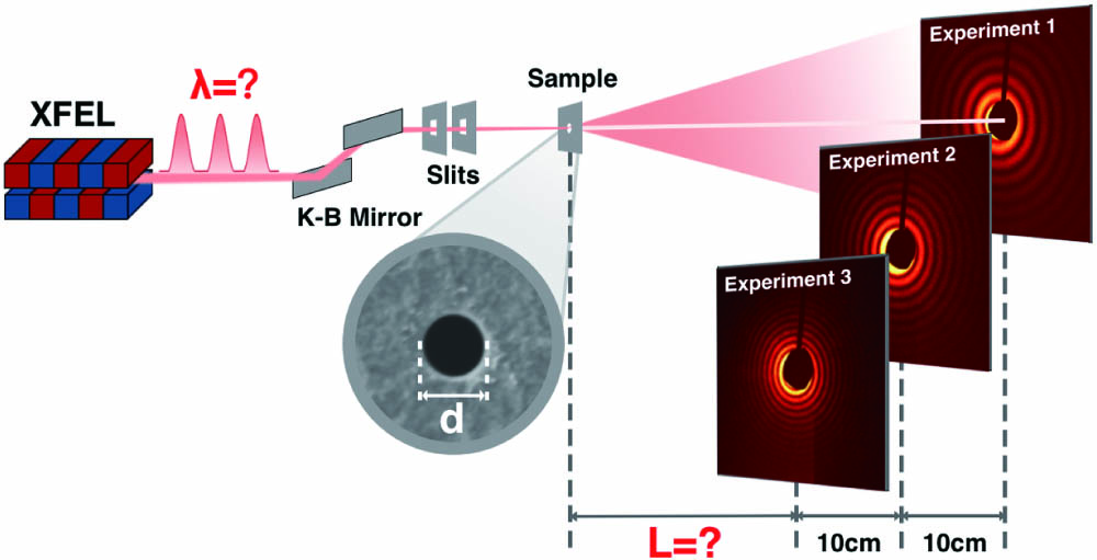
The experiment was conducted at the SXFEL’s CSI end station. The pink branch in the SASE beamline of the SXFEL provides soft X-rays with photon energies ranging from 100 to 620 eV. In this experiment, the X-ray photon energy was set near the N K-edge and the Sc L-edge^[34]. A charge-coupled device X-ray detector (CCD detector, model PI-MTE3:4096B-2) was installed approximately 37 cm downstream of the sample at the CSI end station. The CCD detector was used to collect the single-pulse diffraction patterns. The CCD detector was installed on the XYZ vacuum movement stages, which can be used to adjust the sample-to-detector distance with the $x$-axis and align the detector position with the $y$-axis stage in the horizontal direction and the $z$-axis stage in the vertical direction. The moving resolution of the $x$ axis is 10 µm. An X-ray pulse selector with a maximum operating frequency of 50 Hz was installed upstream from the sample. The pulse selector is triggered by the CCD. By synchronizing the CCD and timing system of the SXFEL and controlling the CCD exposure time, only one pulse can pass through the pulse selector. The pulse selector was not opened until the CCD was ready for the subsequent exposure. Owing to the CCD detector’s limited frame rate, the actual data collection frequency was approximately 0.3 Hz. The experimental setup and method are shown in Fig. 1. The XFEL pulse was focused using K-B mirrors and cleaned with two sets of clean slits installed upstream of the focus. The focus size at the sample position was measured to be approximately 3 µm with full width at half-maximum (FWHM) using the knife-edge scan method^[35]. A standard pinhole with a 1.025 µm diameter, as shown in Fig. 2(a), was mounted on the sample stage at the focus position. The standard pinhole was fabricated using a focused ion beam (FIB) on a 1.5 µm thick Au layer, electroplated on a 100 nm thick ${\mathrm{Si}}_3{\mathrm{N}}_4$ membrane. The pinhole diameter on the light incident side was measured to be approximately 1.025 µm using a scanning electron microscope (SEM), and on the other side, it was approximately 1.057 µm. A smaller side diameter (1.025 µm) was used as the effective diameter. The diameter of the pinhole is smaller than the FWHM of the focal spots. Thus, the incident wave can be considered flat. Owing to the ultrahigh brightness of the XFEL, a single pulse may damage the sample^[36]. To protect the sample, the XFEL pulse intensity was reduced by 2–3 orders of magnitude using a gas attenuator with Ar as the working gas. To protect the CCD from the direct beam, a beam stop with a diameter of 2 mm was installed in front of the CCD chip.

A long working distance microscope with a resolution better than 10 µm is used to locate the XFEL beam position and roughly align the pinhole at focus. The standard pinhole was scanned by attenuated XFEL pulses during the experiment, and the pinhole diffraction patterns were recorded to determine the optimal pinhole position. At this position, the XFEL beam center should be aligned with the pinhole center. Three hundred diffraction patterns were recorded at this position. By moving the vacuum linear movement stage (Model: XA16F-L23-3G, Kohzu Precision), on which the detector was mounted, the detector was moved upstream by 10 and 20 cm from its original position, and 300 single-pulse diffraction patterns were recorded at each position. These three positions were designated as 1/2/3, which corresponds to experiments 1/2/3. The mean wavelength $\lambda$ for each pulse in SASE mode varies, but the jitter is minimal. In contrast, the variation in the sample-to-detector distance, $\mathrm{\Delta }L$, is relatively large. Therefore, Eqs. (6) and (7) are still applicable. The shape of the diffraction pattern remains nearly unchanged throughout the experiment, indicating that the samples are undamaged. Figures 2(b)–2(d) show the characteristic single-pulse diffraction patterns at these three positions. Figure 2(e) shows the power spectral density (PSD) of the three diffraction patterns shown in Figs. 2(b)–2(d). The selected patterns exhibited a good signal-to-noise ratio (SNR) at high diffraction orders. Equation (4) applies to the third and higher diffraction peaks in experiment 1/2/3. This pinhole diffraction method uses three to six peaks following the third diffraction peak in each diffraction pattern. However, because of beam position and pulse energy fluctuations, only single-shot diffraction patterns with high SNR and intensity can be used to calculate the photon energy and sample-to-detector distance. In this study, diffraction patterns with high intensity and visible sixth or higher diffraction rings were selected for characterization. A total of 61 diffraction patterns with high SNR were selected for all the three experiments, and three to six peaks were extracted from each pattern. Each peak was fitted to determine its peak position in the subpixel to calculate the peak period. As shown in Fig. 3(a), the peak spacings and their respective positions were fitted linearly using the least squares method. The wavelength obtained by fitting is $\lambda =3.05\pm 0.01\mathrm{nm}$, which corresponds to the mean photon energy of 406.5 eV. The sample-to-detector distance was calculated as $L=16.61\pm 0.03\mathrm{cm}$.

By measuring a large number of single-shot diffraction patterns and applying statistical analysis, the photon energy jitter of the SASE mode can be calculated, pulse by pulse^[37]. The photon energy of each pulse was calculated using the fitted distance from the sample to the detector, as shown in Fig. 3(b). For the pinhole diffraction method, the calculated photon energy represents the mean photon energy within the XFEL bandwidth because the photons within the bandwidth would contribute to the diffraction patterns. However, the single-pulse photon energy bandwidth cannot be calculated. The photon energy jitter ${\xi }_E$ can be expressed as the root mean square (RMS) of the photon energy variation as follows: $${\xi }_E=\sqrt{\frac{1}{n}{\sum }_n{(E_n-\overline{E})}^2},$$(8)where $E_n$ represents the mean photon energy of each pulse and $\overline{E}$ denotes the mean photon energy of all pulses. ${\xi }_E$ of the pinhole diffraction method was calculated to be 1.39 eV.

XAS is commonly used to calibrate X-ray photon energy. To validate the calculated X-ray photon energy from standard pinhole diffraction, the X-ray absorption spectrum of a 600 nm-thick ${\mathrm{Si}}_3{\mathrm{N}}_4$ membrane was measured at the N K-edge. Simultaneously, the primary absorption peak of nitrogen in the XAS spectrum was used to calibrate the X-ray photon energy. The photon energy can be varied by adjusting the undulator gap. As the photon energy bandwidth of SASE mode is approximately 3 eV (FWHM) at about 404 eV, the X-ray photon energy was scanned using a step of approximately 3 eV during the XAS experiment. Thus, smaller steps will not improve the quality of the XAS. At each photon energy point, the incident pulse energy was measured with a gas monitor detector (GMD) and the transmitted X-ray intensity after the ${\mathrm{Si}}_3{\mathrm{N}}_4$ membrane was recorded by an X-ray photodiode (PD) installed just behind the ${\mathrm{Si}}_3{\mathrm{N}}_4$ membrane. Twelve energy points were measured to obtain the XAS profile. For each X-ray photon energy point, the incident X-ray intensity $I_0$ was normalized by the GMD, and the transmitted X-ray intensity $I_t$ was recorded by the PD. The optical density (OD) can be obtained as follows: $$\mathrm{OD}=-\ln (I_t/I_0).$$(9)

The red line in Fig. 4(a) shows the experimental absorption spectrum, while the blue line represents the reference one^[38]. The photon energy was calibrated by comparing it to the N K-edge of ${\mathrm{Si}}_3{\mathrm{N}}_4$ at about 404 eV, as shown in Fig. 4(a). As the peak width of N K-edge in reference XAS is about 13 eV, the XAS profile as shown in Fig. 4(a) could be measured with an interval of 3 eV. The undulator gap parameter used in the pinhole diffraction method is between the undulator gap used at experiment numbers 9 and 10 in Table 1, and photon energy 406.5 eV measured by diffraction method is also located between 404.8 and 408.6 eV. Therefore, the absorption spectrum shows good consistency with the proposed pinhole diffraction method.

Simultaneously, a spectrometer was used to collect 50 single-pulse spectral data points at each photon energy point. However, the XFEL does not lase during some pulses, so the signals from these pulses are eliminated, potentially leaving fewer than 50 usable spectral signals. The curves in Fig. 4(b) show the normalized results of the average spectra at 12 different photon energy points, which correspond to the experiment numbers 1 to 12 and average photon energies ranging from 381.9 to 414.8 eV in Table 1. The photon energy jitter between pulses can be obtained by calculating the average photon energy $E_n$ per pulse. The normalized histogram of each photon energy point in Fig. 4(b) shows the photon energy statistics for all pulses at that photon energy point. In addition, the photon energy jitter ${\xi }_E$ for each photon energy point was calculated using Eq. (8). However, because the number of single-pulse spectra in experiments 9 and 11 is small, the photon energy jitter is abnormal, as shown in Table 1. The photon energy statistics for all pulses from spectral results, ${\xi }_E$ can be determined as 0.84 eV, as listed in Table 1, which is similar to the photon energy jitter measured by pinhole diffraction method result.

Using the pinhole diffraction method, the average X-ray photon energy was calculated to be 406.5 eV with a photon energy jitter of 1.39 eV, and the sample-to-detector distance of 16.61 cm was determined accurately. The X-ray photon energy calculations obtained using the pinhole diffraction method were compared with the ${\mathrm{Si}}_3{\mathrm{N}}_4$ XAS profile. In addition, the pinhole diffraction method does not require measuring the photon energy at the absorption edges of specific elements, nor does it require a photon energy scan. By measuring the photon energy pulse by pulse, the photon energy jitter can also be calculated without inserting the single-pulse spectrometer to beamline. Besides, spectrometers and XAS cannot measure sample-to-detector distance, which is a very important parameter for both scattering and imaging experiments. This pinhole diffraction method is straightforward and requires minimal prior knowledge. This method accurately measures the sample-to-detector distance as well as the photon energy of each pulse.

In addition, the pinhole diffraction method can be optimized in the future. For example, more precise measurements of a pinhole’s roundness and diameter are conducive to the calculation of photon energy. If a square hole is considered as the sample, the diffraction pattern no longer depends on the approximation of Eq. (4). The intensity distribution of the beam may also cause a shift in the position of the diffraction peak; the selection of a high-intensity pattern can reduce this effect. Furthermore, the limitation of pinhole diffraction method with a standard pinhole as a sample cannot measure the spectrum or bandwidth of individual pulses, whereas it may be possible to measure the spectrum using a transmission grating as a sample. Finally, in the future, the pinhole diffraction method will be able to accurately characterize the photon energy and photon energy jitter of XFELs conveniently, which can be used to calibrate the spectrometer, analyze imaging results, and optimize the light source.